Differential Equations: An Introduction to Modern Methods and Applications
3rd Edition
ISBN: 9781118531778
Author: James R. Brannan, William E. Boyce
Publisher: WILEY
bartleby

Concept explainers

bartleby

Videos

Textbook Question
Book Icon
Chapter 2.P3, Problem 1P

Simulate five sample trajectories of Eq. ( 1 ) for the following parameter values and plot the trajectories on the same set of coordinate axes: μ = 0.12 , σ = 0.1 , T = 1 , s = $ 40 , N = 254 . Then repeat the experiment using the value σ = 0.25 for the volatility. Do the sample trajectories generated in the latter case appear to exhibit a greater degree of variability in their behaviour?

Hint: For the ε n ’s it is permissible to use a random number generator that creates normally distributed random numbers with mean 0 and variance 1 .

Equation ( 1 ) : The discrete model for change in the price of a stock over a time interval [ 0 , T ] is

S n + 1 = S n + μ S n Δ t + σ S n n + 1 Δ t , S 0 = s ,

where S n = S ( t n ) is the stock price at time t n = n Δ t , n = 0 , . . . , N 1 , Δ t = T / N , μ is the annual growth rate of the stock, and σ is a measure of the stock’s annual price volatility or tendency to fluctuate.

Expert Solution & Answer
Check Mark
To determine

The five sample trajectories of the equation Sn+1=Sn+μSnΔt+σSnn+1Δt,S0=s over the time interval [0,T] and plot the trajectories on the same set of coordinate axes, where the parameter values are μ=0.12,σ=0.1,T=1,s=$40,N=254 and repeat the experiment using the value σ=0.25 also determine whether the sample trajectories for σ=0.25 has a greater degree of variability or not as compared to σ=0.1.

Answer to Problem 1P

Solution:

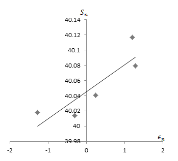
The five sample trajectories for σ=0.1 is

S1=40.014117,S2=40.017659,S3=40.04040,S4=40.07913 and S5=40.1167.

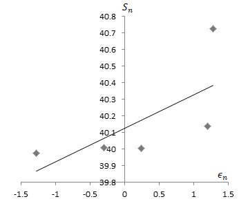
The five sample trajectories for σ=0.25 is

S1=40.007,S2=39.97596,S3=40.004,S4=40.072587 and S5=40.13822.

For σ=0.25, the degree of variability is greater than the degree of variability for σ=0.1.

Explanation of Solution

Given information:

The discrete model for change in the price of a stock over a time interval [0,T] is Sn+1=Sn+μSnΔt+σSnn+1Δt,S0=s, where Sn=S(tn) is the stock price at time tn=nΔt,n=0,...,N1,Δt=T/N,μ is the annual growth rate of the stock, and σ is a measure of the stock’s annual price volatility.

The parameter values are μ=0.12,σ=0.1,T=1,s=$40,N=254.

Highly volatile have a large value for σ.

A sequence of numbers n can easily be created by using one of the random number generators.

Explanation:

The discrete model for change in the price of a stock over a time interval [0,T] is Sn+1=Sn+μSnΔt+σSnn+1Δt,S0=s (1)

Where Sn=S(tn) is the stock price at time tn=nΔt,n=0,...,N1,Δt=T/N.

The parameter values are μ=0.12,σ=0.1,T=1,s=$40,N=254.

Substitute the above values in the equation (1)

Sn+1=Sn+0.12SnΔt+0.1Snn+1Δt.

Here, Δt=T/N

Δt=1/254=0.0039.

Thus, equation (1) becomes,

Sn+1=Sn+0.12Sn×0.0039+0.1Snn+1×0.0039

Sn+1=Sn+0.00047Sn+0.00039Snn+1

Sn+1=1.00047Sn+0.00039Snn+1 ... (2)

Now, to find the value of n for five sample trajectories,

By using the computer technology,

For n=0,1=0.30023

Substitute the values in equation (2)

S0+1=1.00047S0+0.00039S00+1

S1=1.00047s+0.00039s1

S1=1.00047×40+0.00039×40×(0.30023)

S1=40.01880.004683

S1=40.014117.

For n=1,2=1.27768

Substitute the values in equation (2)

S1+1=1.00047S1+0.00039S11+1

S2=1.00047S1+0.00039S12

S2=1.00047×40.0188+0.00039×40.0188×(1.27768)

S2=40.03760.019941

S2=40.017659.

For n=2,3=0.244257

Substitute the values in equation (2)

S2+1=1.00047S2+0.00039S22+1

S3=1.00047S2+0.00039S23

S3=1.00047×40.017659+0.00039×40.017659×(0.244257)

S3=40.0365+0.0038121

S3=40.04040.

For n=3,4=1.276474

Substitute the values in equation (2)

S3+1=1.00047S3+0.00039S33+1

S4=1.00047S3+0.00039S34

S4=1.00047×40.04040+0.00039×40.04040×(1.276474)

S4=40.0592+0.019933

S4=40.07913.

For n=4,5=1.19835

Substitute the values in equation (2)

S4+1=1.00047S4+0.00039S44+1

S5=1.00047S4+0.00039S45

S5=1.00047×40.07913+0.00039×40.07913×(1.19835)

S5=40.09797+0.018731

S5=40.1167.

Hence, the graph of trajectories for σ=0.1 as shown in below figure:

Differential Equations: An Introduction to Modern Methods and Applications, Chapter 2.P3, Problem 1P , additional homework tip  1

Now, for the value σ=0.25,

Sn+1=Sn+0.12SnΔt+0.25Snn+1Δt.

Here, Δt=T/N

Δt=1/254=0.0039.

Thus, equation (1) becomes,

Sn+1=Sn+0.12Sn×0.0039+0.25Snn+1×0.0039

Sn+1=Sn+0.00047Sn+0.000975Snn+1

Sn+1=1.00047Sn+0.000975Snn+1 ... (3)

Now, to find the value of n for five sample trajectories,

By using computer technology,

For n=0,1=0.30023

Substitute the values in equation (3)

S0+1=1.00047S0+0.000975S00+1

S1=1.00047s+0.000975s1

S1=1.00047×40+0.000975×40×(0.30023)

S1=40.01880.0117

S1=40.007.

For n=1,2=1.27768

Substitute the values in equation (3)

S1+1=1.00047S1+0.000975S11+1

S2=1.00047S1+0.000975S12

S2=1.00047×40.007+0.000975×40.007×(1.27768)

S2=40.02580.049838

S2=39.97596.

For n=2,3=0.244257

Substitute the values in equation (3)

S2+1=1.00047S2+0.000975S22+1

S3=1.00047S2+0.000975S23

S3=1.00047×39.97596+0.000975×39.97596×(0.244257)

S3=39.9947+0.00952

S3=40.004.

For n=3,4=1.276474

Substitute the values in equation (2)

S3+1=1.00047S3+0.000975S33+1

S4=1.00047S3+0.000975S34

S4=1.00047×40.004+0.000975×40.004×(1.276474)

S4=40.0228+0.049787

S4=40.072587.

For n=4,5=1.19835

Substitute the values in equation (3)

S4+1=1.00047S4+0.000975S44+1

S5=1.00047S4+0.000975S45

S5=1.00047×40.072587+0.000975×40.072587×(1.19835)

S5=40.0914+0.04682

S5=40.13822.

The graph of trajectories for σ=0.25 is as shown in the below figure:

Differential Equations: An Introduction to Modern Methods and Applications, Chapter 2.P3, Problem 1P , additional homework tip  2

Since the approximation in the graph of trajectories for σ=0.1 is better than the graph of trajectories for σ=0.25.

Therefore, for σ=0.25, the degree of variability is greater than the degree of variability for σ=0.1.

Want to see more full solutions like this?

Subscribe now to access step-by-step solutions to millions of textbook problems written by subject matter experts!
Students have asked these similar questions
In a volatile housing market, the overall value of a home can be modeled by V(x) = 415x² - 4600x + 200000, where V represents the value of the home and x represents each year after 2020. Part A: Find the vertex of V(x). Show all work. Part B: Interpret what the vertex means in terms of the value of the home.
Show all work to solve 3x² + 5x - 2 = 0.
Two functions are given below: f(x) and h(x). State the axis of symmetry for each function and explain how to find it. f(x) h(x) 21 5 4+ 3 f(x) = −2(x − 4)² +2 + -5 -4-3-2-1 1 2 3 4 5 -1 -2 -3 5

Chapter 2 Solutions

Differential Equations: An Introduction to Modern Methods and Applications

Ch. 2.1 - In each of Problems 1 through 12, solve the given...Ch. 2.1 - In each of Problems through , solve the given...Ch. 2.1 - In each of Problems through : (a) Find the...Ch. 2.1 - In each of Problems through : (a) Find the...Ch. 2.1 - In each of Problems through : (a) Find the...Ch. 2.1 - In each of Problems through : (a) Find the...Ch. 2.1 - In each of Problems through : (a) Find the...Ch. 2.1 - In each of Problems through : (a) Find the...Ch. 2.1 - In each of Problems through : (a) Find the...Ch. 2.1 - In each of Problems 13 through 28: (a) Find the...Ch. 2.1 - In each of Problems through : (a) Find the...Ch. 2.1 - In each of Problems 13 through 28: (a) Find the...Ch. 2.1 - In each of Problems through : (a) Find the...Ch. 2.1 - In each of Problems 13 through 28: (a) Find the...Ch. 2.1 - In each of Problems 13 through 28: (a) Find the...Ch. 2.1 - In each of Problems through : (a) Find the...Ch. 2.1 - In each of Problems 13 through 28: (a) Find the...Ch. 2.1 - In each of Problems through : (a) Find the...Ch. 2.1 - In Problems through , obtain the requested...Ch. 2.1 - In Problems 29 through 36, obtain the requested...Ch. 2.1 - In Problems through , obtain the requested...Ch. 2.1 - In Problems 29 through 36, obtain the requested...Ch. 2.1 - In Problems through , obtain the requested...Ch. 2.1 - In Problems 29 through 36, obtain the requested...Ch. 2.1 - In Problems through , obtain the requested...Ch. 2.1 - In Problems 29 through 36, obtain the requested...Ch. 2.1 - Solve the equation dydx=ay+bcy+d, where a,b,c, and...Ch. 2.2 - In each of Problems 1 through 12: Draw a direction...Ch. 2.2 - In each of Problems 1 through 12: Draw a...Ch. 2.2 - In each of Problems 1 through 12: Draw a...Ch. 2.2 - In each of Problems 1 through 12: Draw a...Ch. 2.2 - In each of Problems 1 through 12: Draw a...Ch. 2.2 - In each of Problems 1 through 12: Draw a...Ch. 2.2 - In each of Problems 1 through 12: Draw a direction...Ch. 2.2 - In each of Problems 1 through 12: Draw a direction...Ch. 2.2 - In each of Problems 1 through 12: Draw a direction...Ch. 2.2 - In each of Problems 1 through 12: Draw a direction...Ch. 2.2 - In each of Problems 1 through 12: Draw a direction...Ch. 2.2 - In each of Problems 1 through 12: Draw a direction...Ch. 2.2 - In each of Problems 13 through 20, find the...Ch. 2.2 - In each of Problems 13 through 20, find the...Ch. 2.2 - In each of Problems 13 through 20, find the...Ch. 2.2 - In each of Problems 13 through 20, find the...Ch. 2.2 - In each of Problems 13 through 20, find the...Ch. 2.2 - In each of Problems 13 through 20, find the...Ch. 2.2 - In each of Problems 13 through 20, find the...Ch. 2.2 - In each of Problems 21 through 23: Draw a...Ch. 2.2 - In each of Problems 21 through 23: Draw a...Ch. 2.2 - In each of Problems 21 through 23: Draw a...Ch. 2.2 - In each of Problems 21 through 23: Draw a...Ch. 2.2 - In each of Problems 24 through 26: Draw a...Ch. 2.2 - In each of Problems 24 through 26: Draw a...Ch. 2.2 - In each of Problems 24 through 26: Draw a...Ch. 2.2 - Consider the initial value problem Find the...Ch. 2.2 - Consider the initial value problem Find the value...Ch. 2.2 - Consider the initial value problem...Ch. 2.2 - Find the value of y0 for which the solution of the...Ch. 2.2 - Consider the initial value problem Find the value...Ch. 2.2 - Show that all solutions of [Eq. (36) of the text]...Ch. 2.2 - Show that if andare positive constants, and b is...Ch. 2.2 - In each of Problems 34 through 37, construct a...Ch. 2.2 - In each of Problems 34 through 37, construct a...Ch. 2.2 - In each of Problems 34 through 37, construct a...Ch. 2.2 - In each of Problems 34 through 37, construct a...Ch. 2.2 - Consider the initial value problem...Ch. 2.2 - Variation of Parameters. Consider the following...Ch. 2.2 - In each of Problems 40 through 43 use the method...Ch. 2.2 - In each of Problems 40 through 43 use the method...Ch. 2.2 - In each of Problems 40 through 43 use the method...Ch. 2.2 - In each of Problems 40 through 43 use the method...Ch. 2.3 - Consider a tank used in certain hydrodynamic...Ch. 2.3 - A tank initially contains 200L of pure water. A...Ch. 2.3 - A tank originally contains gal of fresh water....Ch. 2.3 - A tank with a capacity of originally contains of...Ch. 2.3 - A tank contains of water and of salt. Water...Ch. 2.3 - Suppose that a tank containing a certain liquid...Ch. 2.3 - An outdoor swimming pool loses 0.05 of its water...Ch. 2.3 - Cholesterol is produced by the body for the...Ch. 2.3 - Imagine a medieval world. In this world a Queen...Ch. 2.3 - Suppose an amount is invested at an annual rate...Ch. 2.3 - A young person with no initial capital invests ...Ch. 2.3 - A homebuyer can afford to spend no more than on...Ch. 2.3 - A recent college graduate borrows 100,000 at an...Ch. 2.3 - A Difference Equation. In this problem, we...Ch. 2.3 - An important tool in archaeological research is...Ch. 2.3 - The population of mosquitoes in a certain area...Ch. 2.3 - Suppose that a certain population has growth rate...Ch. 2.3 - Suppose that a certain population satisfies the...Ch. 2.3 - Newtons law of cooling states that the temperature...Ch. 2.3 - Heat transfer from a body to its surrounding by...Ch. 2.3 - Consider a lake of constant volume containing at...Ch. 2.3 - A ball with mass 0.25 kg is thrown upward with...Ch. 2.3 - Assume that conditions are as Problemexcept that...Ch. 2.3 - Assume that conditions are as in Problem 22 except...Ch. 2.3 - A skydiver weighing 180 lb (including equipment)...Ch. 2.3 - A rocket sled having an initial speed of mi/h is...Ch. 2.3 - A body of constant mass is projected vertically...Ch. 2.3 - Prob. 28PCh. 2.3 - Prob. 29PCh. 2.3 - A mass of 0.40 kg is dropped from rest in a medium...Ch. 2.3 - Suppose that a rocket is launched straight up from...Ch. 2.3 - Let and , respectively, be the horizontal and...Ch. 2.3 - A more realistic model (than that in Problem 32)...Ch. 2.3 - Brachistochrone Problem. One of the famous...Ch. 2.4 - Existence and uniqueness of Solutions. In each of...Ch. 2.4 - Existence and uniqueness of Solutions. In each of...Ch. 2.4 - Existence and uniqueness of Solutions. In each of...Ch. 2.4 - Existence and uniqueness of Solutions. In each of...Ch. 2.4 - Existence and uniqueness of Solutions. In each of...Ch. 2.4 - Existence and uniqueness of Solutions. In each of...Ch. 2.4 - In each of Problem through, state where in -...Ch. 2.4 - In each of Problem through, state where in -...Ch. 2.4 - In each of Problem through, state where in -...Ch. 2.4 - In each of Problem 7 through 12, state where in...Ch. 2.4 - In each of Problem through, state where in -...Ch. 2.4 - In each of Problem through, state where in -...Ch. 2.4 - Consider the initial value problem y=y1/3,y(0)=0...Ch. 2.4 - Verify that both and are solutions of the...Ch. 2.4 - Dependence of Solutions on Initial Conditions. In...Ch. 2.4 - Dependence of Solutions on Initial Conditions. In...Ch. 2.4 - Dependence of Solutions on Initial Conditions. In...Ch. 2.4 - Dependence of Solutions on Initial Conditions. In...Ch. 2.4 - In each of Problem 19 through 22, draw a direction...Ch. 2.4 - In each of Problem 19 through 22, draw a direction...Ch. 2.4 - In each of Problem through, draw a direction...Ch. 2.4 - In each of Problem through, draw a direction...Ch. 2.4 - Show that is a solution of and that is also a...Ch. 2.4 - Show that if y=(t) is a solution of y+p(t)y=0,...Ch. 2.4 - Let y=y1(t) be a solution of y+p(t)y=0, (i) and...Ch. 2.4 - Show that the solution (7) of the general...Ch. 2.4 - Discontinuous Coefficients. Linear differential...Ch. 2.4 - Discontinuous Coefficients. Linear differential...Ch. 2.4 - Consider the initial value problem ...Ch. 2.5 - Suppose that a certain population obeys the...Ch. 2.5 - Another equation that has been used to model...Ch. 2.5 - (a) Solve the Gompertz equation subject to the...Ch. 2.5 - A pond forms as water collects in a conical...Ch. 2.5 - Consider a cylindrical water tank of constant...Ch. 2.5 - Epidemics. The use of mathematical methods to...Ch. 2.5 - Epidemics. The use of mathematical methods to...Ch. 2.5 - Epidemics. The use of mathematical methods to...Ch. 2.5 - Chemical Reactions. A second order chemical...Ch. 2.5 - Bifurcation Points. For an equation of the form...Ch. 2.5 - Bifurcation Points. For an equation of the form ...Ch. 2.5 - Bifurcation Points. For an equation of the form...Ch. 2.6 - Exact Equations. In each of Problem through...Ch. 2.6 - Exact Equations. In each of Problem 1 through 12:...Ch. 2.6 - Exact Equations. In each of Problem through...Ch. 2.6 - Exact Equations. In each of Problem through...Ch. 2.6 - Exact Equations. In each of Problem 1 through 12:...Ch. 2.6 - Exact Equations. In each of Problem 1 through 12:...Ch. 2.6 - Exact Equations. In each of Problem through...Ch. 2.6 - Exact Equations. In each of Problem 1 through 12:...Ch. 2.6 - Exact Equations. In each of Problem 1 through 12:...Ch. 2.6 - Exact Equations. In each of Problem through...Ch. 2.6 - Exact Equations. In each of Problem through...Ch. 2.6 - Exact Equations. In each of Problem through...Ch. 2.6 - In each of Problem and , solve the given initial...Ch. 2.6 - In each of Problem 13 and 14, solve the given...Ch. 2.6 - In each of Problem 15 and 16, find the value of b...Ch. 2.6 - In each of Problem 15 and 16, find the value of b...Ch. 2.6 - Assume that Eq. (6) meets the requirements of...Ch. 2.6 - Show that any separable equation is also exact. Ch. 2.6 - Integrating Factor. In each of Problem through...Ch. 2.6 - Integrating Factor. In each of Problem through...Ch. 2.6 - Integrating Factor. In each of Problem 19 through...Ch. 2.6 - Integrating Factor. In each of Problem through...Ch. 2.6 - Show that if (NxMy)/M=Q, where Q is function of y...Ch. 2.6 - Show that if , where depends on the quantity ...Ch. 2.6 - In each of Problem 25 through 31: Find an...Ch. 2.6 - In each of Problem through: Find an integrating...Ch. 2.6 - In each of Problem 25 through 31: Find an...Ch. 2.6 - In each of Problem 25 through 31: Find an...Ch. 2.6 - In each of Problem through: Find an integrating...Ch. 2.6 - In each of Problem 25 through 31: Find an...Ch. 2.6 - In each of Problem 25 through 31: Find an...Ch. 2.6 - Use the integrating factor (x,y)=[xy(2x+y)]1 to...Ch. 2.7 - Homogeneous Differential Equations. In each of...Ch. 2.7 - Homogeneous Differential Equations. In each of...Ch. 2.7 - Homogeneous Differential Equations. In each of...Ch. 2.7 - Homogeneous Differential Equations. In each of...Ch. 2.7 - Homogeneous Differential Equations. In each of...Ch. 2.7 - Homogeneous Differential Equations. In each of...Ch. 2.7 - Homogeneous Differential Equations. In each of...Ch. 2.7 - Homogeneous Differential Equations. In each of...Ch. 2.7 - Homogeneous Differential Equations. In each of...Ch. 2.7 - Homogeneous Differential Equations. In each of...Ch. 2.7 - In problem 11 and 12, solve the given initial...Ch. 2.7 - In problem and, solve the given initial value...Ch. 2.7 - In each of Problems 13 through 22: Write the...Ch. 2.7 - In each of Problems through: Write the Bernoulli...Ch. 2.7 - In each of Problems through: Write the Bernoulli...Ch. 2.7 - In each of Problems through: Write the Bernoulli...Ch. 2.7 - In each of Problems through: Write the Bernoulli...Ch. 2.7 - In each of Problems 13 through 22: Write the...Ch. 2.7 - In each of Problems through: Write the Bernoulli...Ch. 2.7 - In each of Problems through: Write the Bernoulli...Ch. 2.7 - In each of Problems 13 through 22: Write the...Ch. 2.7 - In each of Problems through: Write the Bernoulli...Ch. 2.7 - A differential equation of the form...Ch. 2.7 - Mixed Practice. In each of Problems 24 through 36:...Ch. 2.7 - Mixed Practice. In each of Problems ...Ch. 2.7 - Mixed Practice. In each of Problems ...Ch. 2.7 - Mixed Practice. In each of Problems 24 through 36:...Ch. 2.7 - Mixed Practice. In each of Problems 24 through 36:...Ch. 2.7 - Mixed Practice. In each of Problems ...Ch. 2.7 - Mixed Practice. In each of Problems 24 through 36:...Ch. 2.7 - Mixed Practice. In each of Problems 24 through 36:...Ch. 2.7 - Mixed Practice. In each of Problems ...Ch. 2.7 - Mixed Practice. In each of Problems ...Ch. 2.7 - Mixed Practice. In each of Problems ...Ch. 2.7 - Mixed Practice. In each of Problems ...Ch. 2.7 - Mixed Practice. In each of Problems 24 through 36:...Ch. 2.P1 - Constant Effort Harvesting. At a given level of...Ch. 2.P1 - Constant Yield Harvesting. In this problem, we...Ch. 2.P2 - Derive Eq. (3) from Eqs. (1) and (2) and show that...Ch. 2.P2 - Additional processes due to biotic and abiotic...Ch. 2.P2 - Show that when , the source has an infinite...Ch. 2.P2 - Assume the following values for the parameters;...Ch. 2.P2 - Effects of Partial Source Remediation. Assume...Ch. 2.P3 - Simulate five sample trajectories of Eq. (1) for...Ch. 2.P3 - Use the difference equation (4) to generate an...Ch. 2.P3 - VarianceReduction by Antithetic Variates. A simple...
Knowledge Booster
Background pattern image
Math
Learn more about
Need a deep-dive on the concept behind this application? Look no further. Learn more about this topic, subject and related others by exploring similar questions and additional content below.
Similar questions
SEE MORE QUESTIONS
Recommended textbooks for you
Text book image
College Algebra
Algebra
ISBN:9781938168383
Author:Jay Abramson
Publisher:OpenStax
Text book image
Big Ideas Math A Bridge To Success Algebra 1: Stu...
Algebra
ISBN:9781680331141
Author:HOUGHTON MIFFLIN HARCOURT
Publisher:Houghton Mifflin Harcourt
Text book image
Glencoe Algebra 1, Student Edition, 9780079039897...
Algebra
ISBN:9780079039897
Author:Carter
Publisher:McGraw Hill
Text book image
Algebra & Trigonometry with Analytic Geometry
Algebra
ISBN:9781133382119
Author:Swokowski
Publisher:Cengage
Text book image
Functions and Change: A Modeling Approach to Coll...
Algebra
ISBN:9781337111348
Author:Bruce Crauder, Benny Evans, Alan Noell
Publisher:Cengage Learning
Text book image
College Algebra
Algebra
ISBN:9781305115545
Author:James Stewart, Lothar Redlin, Saleem Watson
Publisher:Cengage Learning
Correlation Vs Regression: Difference Between them with definition & Comparison Chart; Author: Key Differences;https://www.youtube.com/watch?v=Ou2QGSJVd0U;License: Standard YouTube License, CC-BY
Correlation and Regression: Concepts with Illustrative examples; Author: LEARN & APPLY : Lean and Six Sigma;https://www.youtube.com/watch?v=xTpHD5WLuoA;License: Standard YouTube License, CC-BY