Concept explainers
The basic
Where

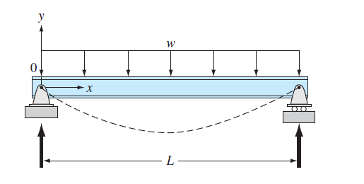
FIGURE P28.27
(a)
To calculate: The deflection of the beam by the finite-difference method with
Answer to Problem 27P
Solution:
The deflection of the beam by the finite-difference method is,
| x | y | y-Analytical |
| 0 | 0 | 0 |
| 24 | ||
| 48 | ||
| 72 | ||
| 96 | ||
| 120 | 0 | 0 |
Explanation of Solution
Given Information:
The differential equation for the elastic curve for a uniformly loaded beam is given as,
Formula to find analytical value,
Where,
The modulus of elasticity,
The moment of inertia,
The values,
Formula used:
The conversion formula,
The value of second order derivative by finite difference method is given as,
Calculation:
Consider the equation,
Rewrite the above equation as,
Substitute the values,
Now, the second order derivative by finite difference method gives,
Therefore,
Put
The boundary condition is,
Put
Substitute
Put
Substitute
Put
Substitute
The matrix form of the above equations is given as below,
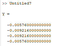
Use MATLAB to find the solution of the above system as below,
Code:
%Write the matrix
A=[-2 1 0 0; 1 -2 1 0; 0 1 -2 1; 0 0 1 -2];
%write the values of rhs
b=[0.002304 0.003456 0.003456 0.002304]';
%find the result
Y=A\b
Output:

Now, for the analytical value, consider the equation
Substitute the values,
Use excel to find the values of y at different values of x as below,
Step 1: Name the column A as x and go to column A2 and put 0 then go to column A3 and write the formula as,
=A2+24
Then, Press enter and drag the column up to
Step 2: Now name the column B as y and go to column B2 andwrite the formula as,
=2.89236*10^(-10)*A2*(120*A2^2-0.5*A2^3-864000)
Step 3: Press enter and drag the column up to
The result obtained as,
| x | y-Analytical |
| 0 | 0 |
| 24 | |
| 48 | |
| 72 | |
| 96 | |
| 120 | 0 |
(b)
To calculate: The deflection of the beam by the shooting method with
Answer to Problem 27P
Solution:
A few values of deflection of the beam by the shooting method is,
| x | y | z |
| 0 | 0 | -1.6E-06 |
| 0.25 | -4.1E-07 | -1.6E-06 |
| 0.5 | -8.2E-07 | -1.6E-06 |
| 0.75 | -1.2E-06 | -1.6E-06 |
| 1 | -1.6E-06 | -1.6E-06 |
| 1.25 | -2E-06 | -1.5E-06 |
| 1.5 | -2.4E-06 | -1.4E-06 |
| 1.75 | -2.8E-06 | -1.4E-06 |
| 2 | -3.2E-06 | -1.3E-06 |
| 2.25 | -3.5E-06 | -1.2E-06 |
| 2.5 | -3.8E-06 | -1.1E-06 |
| 2.75 | -4.1E-06 | -1E-06 |
| 3 | -4.4E-06 | -9E-07 |
Explanation of Solution
Given Information:
The differential equation for the elastic curve for a uniformly loaded beam is given as,
Formula to find analytical value,
Where,
The modulus of elasticity,
The moment of inertia,
The values,
Formula used:
The conversion formula,
Calculation:
Consider the equation,
Rewrite the equation as,
Assume
Substitute the values,
Use VBA program as below to solve the above differential equation as below,
Code:
OptionExplicit
'Create a function find
Subfind()
'declare the variables as integer
Dim n AsInteger, j AsInteger
'declare the variables as double
DimdydxAsDouble, x AsDouble, dy2dx AsDouble, yanalAsDouble, E AsDouble, I AsDouble, w AsDouble, L AsDouble
DimolddydxAsDouble, oldy AsDouble, y AsDouble, h AsDouble
'Set the values of the variables
E =30000
I =800
w =1
L =10
y =0
x =0
h =0.25
dydx=0
'store dydx and analytical solution
dydx= caldydx(w, E, I, L, x)
yanal= caly(w, E, I, L, x)
'use for loop to determine different value of y and y analytical
For j =1 To41
'store the value of y at oldy and dydx in olddydx
oldy = y
olddydx= dydx
'Store d2ydx, dydx and analytical solution
dy2dx = caldy2dx(w, E, I, L, x)
dydx= caldydx(w, E, I, L, x)
yanal= caly(w, E, I, L, x)
'move to the cell b3
Range("b1"). Select
ActiveCell.Value="shooting method"
'Assign name to the columns
ActiveCell.Offset(1,0). Select
ActiveCell.Value="x"
ActiveCell.Offset(0,1). Select
ActiveCell.Value="y"
ActiveCell.Offset(0,1). Select
ActiveCell.Value="z"
ActiveCell.Offset(0,1). Select
ActiveCell.Value="dy2dx"
ActiveCell.Offset(0,1). Select
ActiveCell.Value="y-anal"
'dislay values in cell
Range("b2"). Select
ActiveCell.Offset(j,0). Select
ActiveCell.Value= x
ActiveCell.Offset(0,1). Select
ActiveCell.Value= oldy
ActiveCell.Offset(0,1). Select
ActiveCell.Value= dydx
ActiveCell.Offset(0,1). Select
ActiveCell.Value= dy2dx
ActiveCell.Offset(0,1). Select
ActiveCell.Value= yanal
'Write the next value of x
x = x + h
'Write the next value of y by euler method
y = oldy + olddydx* h
Next
EndSub
'Define d2ydx function
Function caldy2dx(w, E, I, L, x)
'Declare the variables
Dim t AsDouble
'Write the formula
t =((w * L * x)/(2* E * I))-((w * x * x)/(2* E * I))
'Store the value
caldy2dx = t
EndFunction
'Define dydx
Functioncaldydx(w, E, I, L, x)
'Declare the variables
Dim t AsDouble, c AsDouble
'Set the values
c =-0.000001648
'Write the formula
t =((w * L * x * x)/(4* E * I))-((w * x * x * x)/(6* E * I))+ c
'Store the value
caldydx= t
EndFunction
'Define the function caly for analytical value
Functioncaly(w, E, I, L, x)
'Declare the variables
Dim t AsDouble
'Write the formula
t =((w * L * x * x * x)/(12* E * I))-((w * x * x * x * x)/(24* E * I))-((w * L * L * L * x)/(24* E * I))
'Store the value
caly= t
EndFunction
Output:
| shooting method | ||||
| x | y | z | dy2dx | y-anal |
| 0 | 0 | -1.6E-06 | 0 | 0 |
| 0.25 | -4.1E-07 | -1.6E-06 | 5.08E-08 | -4.3E-07 |
| 0.5 | -8.2E-07 | -1.6E-06 | 9.9E-08 | -8.6E-07 |
| 0.75 | -1.2E-06 | -1.6E-06 | 1.45E-07 | -1.3E-06 |
| 1 | -1.6E-06 | -1.6E-06 | 1.88E-07 | -1.7E-06 |
| 1.25 | -2E-06 | -1.5E-06 | 2.28E-07 | -2.1E-06 |
| 1.5 | -2.4E-06 | -1.4E-06 | 2.66E-07 | -2.5E-06 |
| 1.75 | -2.8E-06 | -1.4E-06 | 3.01E-07 | -2.9E-06 |
| 2 | -3.2E-06 | -1.3E-06 | 3.33E-07 | -3.2E-06 |
| 2.25 | -3.5E-06 | -1.2E-06 | 3.63E-07 | -3.6E-06 |
| 2.5 | -3.8E-06 | -1.1E-06 | 3.91E-07 | -3.9E-06 |
| 2.75 | -4.1E-06 | -1E-06 | 4.15E-07 | -4.2E-06 |
| 3 | -4.4E-06 | -9E-07 | 4.38E-07 | -4.4E-06 |
| 3.25 | -4.7E-06 | -7.9E-07 | 4.57E-07 | -4.6E-06 |
| 3.5 | -4.9E-06 | -6.7E-07 | 4.74E-07 | -4.8E-06 |
| 3.75 | -5.1E-06 | -5.5E-07 | 4.88E-07 | -5E-06 |
| 4 | -5.2E-06 | -4.3E-07 | 5E-07 | -5.2E-06 |
| 4.25 | -5.4E-06 | -3E-07 | 5.09E-07 | -5.3E-06 |
| 4.5 | -5.5E-06 | -1.7E-07 | 5.16E-07 | -5.4E-06 |
| 4.75 | -5.6E-06 | -4.2E-08 | 5.2E-07 | -5.4E-06 |
| 5 | -5.6E-06 | 8.81E-08 | 5.21E-07 | -5.4E-06 |
| 5.25 | -5.6E-06 | 2.18E-07 | 5.2E-07 | -5.4E-06 |
| 5.5 | -5.6E-06 | 3.48E-07 | 5.16E-07 | -5.4E-06 |
| 5.75 | -5.5E-06 | 4.76E-07 | 5.09E-07 | -5.3E-06 |
| 6 | -5.4E-06 | 6.02E-07 | 5E-07 | -5.2E-06 |
| 6.25 | -5.3E-06 | 7.26E-07 | 4.88E-07 | -5E-06 |
| 6.5 | -5.2E-06 | 8.46E-07 | 4.74E-07 | -4.8E-06 |
| 6.75 | -5E-06 | 9.62E-07 | 4.57E-07 | -4.6E-06 |
| 7 | -4.8E-06 | 1.07E-06 | 4.38E-07 | -4.4E-06 |
| 7.25 | -4.5E-06 | 1.18E-06 | 4.15E-07 | -4.2E-06 |
| 7.5 | -4.3E-06 | 1.28E-06 | 3.91E-07 | -3.9E-06 |
| 7.75 | -4E-06 | 1.38E-06 | 3.63E-07 | -3.6E-06 |
| 8 | -3.7E-06 | 1.46E-06 | 3.33E-07 | -3.2E-06 |
| 8.25 | -3.3E-06 | 1.54E-06 | 3.01E-07 | -2.9E-06 |
| 8.5 | -3E-06 | 1.61E-06 | 2.66E-07 | -2.5E-06 |
| 8.75 | -2.6E-06 | 1.68E-06 | 2.28E-07 | -2.1E-06 |
| 9 | -2.2E-06 | 1.73E-06 | 1.88E-07 | -1.7E-06 |
| 9.25 | -1.7E-06 | 1.77E-06 | 1.45E-07 | -1.3E-06 |
| 9.5 | -1.3E-06 | 1.8E-06 | 9.9E-08 | -8.6E-07 |
| 9.75 | -8.7E-07 | 1.82E-06 | 5.08E-08 | -4.3E-07 |
| 10 | -4.2E-07 | 1.82E-06 | 0 | 0 |
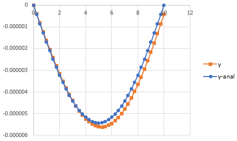
Now, to draw the graph of y and y-analytical follow the step as below,
Step 1: Select the cell from B2 to B43 and cell C2 to C43. Then, go to the Insert and select the scatter with smooth lines from the chart.
Step 2: Select the cell from B2 to B43 and cell F2 to F43. Then, go to the Insert and select the scatter with smooth lines from the chart.
Step 3: Select one of the graphs and paste it on another graph to merge the graphs.
The graph obtained is,

Want to see more full solutions like this?
Chapter 28 Solutions
EBK NUMERICAL METHODS FOR ENGINEERS
Additional Engineering Textbook Solutions
Probability And Statistical Inference (10th Edition)
Introductory Statistics
Finite Mathematics for Business, Economics, Life Sciences and Social Sciences
Elementary and Intermediate Algebra: Concepts and Applications (7th Edition)
A First Course in Probability (10th Edition)
Precalculus: A Unit Circle Approach (3rd Edition)
- Please ensure that all parts of the question are answered thoroughly and clearly. Include a diagram to help explain answers. Make sure the explanation is easy to follow. Would appreciate work done written on paper. Thank you.arrow_forwardUsing the method of joints, determine the force in each member of the truss shown. Summarize the results on a force summation diagram, and indicate whether each member is in tension or compression. You may want to try the "quick" method hod.16 8m T or C CD CE AB EF BF гид B 6m i force in CE only (change top force to 8kn) 8 KN 8kNarrow_forwardNo chatgpt pls will upvotearrow_forward
- Please ensure that all parts of the question are answered thoroughly and clearly. Include a diagram to help explain answers. Make sure the explanation is easy to follow. Would appreciate work done written on paper. Thank you.arrow_forwardI just need help with f and garrow_forwardPlease ensure that all parts of the question are answered thoroughly and clearly. Include a diagram to help explain answers. Make sure the explanation is easy to follow. Would appreciate work done written on paper. Thank you.arrow_forward
- You are coming home hungry and look in your fridge. You find: 1 roll and 2 slices of bread, a jar ofpeanut butter, one single serve package each of mayo and mustard, a can of cheezewhiz, some slicedham, and some sliced turkey. How many different types of (edible) sandwiches can you make? Writedown any assumptions (order matters or not, repetitons allowed or not).arrow_forwardAlready got wrong chatgpt answer Plz don't use chatgpt answer will upvotearrow_forward7. Suppose that X is a set, that I is a nonempty set, and that for each i Є I that Yi is a set. Suppose that I is a nonempty set. Prove the following:2 (a) If Y; CX for all i EI, then Uiel Yi C X. ¹See Table 4.8.1 in zyBooks. Recall: Nie X₁ = Vi Є I (x = X₁) and x = Uier X₁ = i Є I (x Є Xi). (b) If XCY; for all i Є I, then X Ciel Yi. (c) U(x)=xnUY. iЄI ΕΙarrow_forward
- 8. For each of the following functions, determine whether or not it is (i) injective and/or (ii) surjective. Justify why or why not. (a) fiZZ defined by fi(n) = 2n. (b) f2 RR defined by f2(x) = x² − 4x+7. : (c) f3 Z {0, 1} defined by f3(n) = 0 if n is even and f3(n) = 1 if n is odd. (d) f4 Z N defined by f4(n) = 2n if n > 0 and f4(n) = -2n-1 if n < 0.arrow_forward2. Disprove the following by finding counterexamples: 3. (a) For all sets A and B, AU (BNA) = B. (b) For all sets A, B, and C, ANBCC if and only if ACC and B C C. Suppose A and B are subsets of a universal set U. Using the set identities¹ prove the following: (a) (ANB) U(ANB) = B (b) A (BA) = Aarrow_forwardNo chatgpt pls will upvotearrow_forward
 College Algebra (MindTap Course List)AlgebraISBN:9781305652231Author:R. David Gustafson, Jeff HughesPublisher:Cengage Learning
