Chapter 28, Problem 15P

To determine

To calculate: The concentration of each reactant as the function of distance by using the finite difference approach, and apply centred finite-difference approximations with $\Delta x=0.05\text{ m}$.

Answer to Problem 15P

Solution:

The concentration of each reactant as the function of distance is,

The below plot shows the distance versus reactant.

Explanation of Solution

Given Information:

The series of first order, liquid phase reactions is,

$A\stackrel{k_1}{\to }B\stackrel{k_2}{\to }C$

The second order ODEs by using the steady-state mass balance.

$\begin{array}{l}D\frac{d^2{c}_a}{d{x}^2}-U\frac{d{c}_a}{dx}-k_1{c}_a=0\\ D\frac{d^2{c}_b}{d{x}^2}-U\frac{d{c}_b}{dx}+k_1{c}_a-k_2{c}_b=0\\ D\frac{d^2{c}_c}{d{x}^2}-U\frac{d{c}_c}{dx}+k_2{c}_b=0\end{array}$

Here, $c$ is the concentration $\left(\text{mol/L}\right)$, $x$ is the distance $\left(\text{m}\right)$, $D$ is the dispersion coefficient $\left(\text{0}{\text{.1 m}}^{\text{2}}\text{/min}\right)$, $U$ is the velocity $\left(\text{1 m/min}\right)$, $k_1$ is the reaction rate $\left(3/\min \right)$, $k_2$ is the reaction rate $\left(1/\min \right)$.

Refer to the Prob 28.14, the Danckwerts boundary conditions is,

$U{c}_{in}=Uc\left(x=0\right)-D\frac{dc}{dx}\left(x=0\right)$

$\frac{dc}{dx}\left(x=L\right)=0$

Here, $c_{a,\text{in}}$ is the concentration in the inflow $\left(10\text{ mol/L}\right)$, and $L$ is the length of the reactor $\left(0.5\text{ m}\right)$.

$\Delta x=0.05\text{ m}$

Formula used:

The finite divided difference formula is,

$f^{″}\left(x_0\right)=\frac{c_{i-1}-2c_i+c_{i+1}}{\Delta x^2}$

Calculation:

Recall the ordinary differential equations,

$\begin{array}{l}D\frac{d^2{c}_a}{d{x}^2}-U\frac{d{c}_a}{dx}-k_1{c}_a=0\\ D\frac{d^2{c}_b}{d{x}^2}-U\frac{d{c}_b}{dx}+k_1{c}_a-k_2{c}_b=0\\ D\frac{d^2{c}_c}{d{x}^2}-U\frac{d{c}_c}{dx}+k_2{c}_b=0\end{array}$

Substitute the finite divided difference formula in the above differential equations.

$\begin{array}{l}D\left(\frac{c_{a,i-1}-2c_{a,i}+c_{a,i+1}}{\Delta x^2}\right)-U\left(\frac{c_{a,i+1}-c_{a,i-1}}{2\Delta x}\right)-k_1{c}_{a,i}=0\\ D\left(\frac{c_{b,i-1}-2c_{b,i}+c_{b,i+1}}{\Delta x^2}\right)-U\left(\frac{c_{b,i+1}-c_{b,i-1}}{2\Delta x}\right)+k_1{c}_{a,i}-k_2{c}_{b,i}=0\\ D\left(\frac{c_{c,i-1}-2c_{c,i}+c_{c,i+1}}{\Delta x^2}\right)-U\left(\frac{c_{c,i+1}-c_{c,i-1}}{2\Delta x}\right)+k_2{c}_{b,i}=0\end{array}$

Substitute $\left(\text{0}{\text{.1 m}}^{\text{2}}\text{/min}\right)$ for $D$, $\left(\text{1 m/min}\right)$ for $U$, $0.05\text{ m}$ for $\Delta x$, $\left(3/\min \right)$ for $k_1$, and $\left(1/\min \right)$ for $k_2$ yield unit.

$\begin{array}{l}\left(\text{0}\text{.1}\right)\left(\frac{c_{a,i-1}-2c_{a,i}+c_{a,i+1}}{{\left(0.05\right)}^2}\right)-\left(\text{1}\right)\left(\frac{c_{a,i+1}-c_{a,i-1}}{2\left(0.05\right)}\right)-\left(3\right)c_{a,i}=0\\ \left(\text{0}\text{.1}\right)\left(\frac{c_{b,i-1}-2c_{b,i}+c_{b,i+1}}{{\left(0.05\right)}^2}\right)-\left(\text{1}\right)\left(\frac{c_{b,i+1}-c_{b,i-1}}{2\left(0.05\right)}\right)+\left(3\right)c_{a,i}-\left(1\right)c_{b,i}=0\\ \left(\text{0}\text{.1}\right)\left(\frac{c_{c,i-1}-2c_{c,i}+c_{c,i+1}}{{\left(0.05\right)}^2}\right)-\left(\text{1}\right)\left(\frac{c_{c,i+1}-c_{c,i-1}}{2\left(0.05\right)}\right)+\left(1\right)c_{b,i}=0\end{array}$

Solve further,

$\begin{array}{l}-\text{50}{c}_{a,i-1}+83c_{a,i}-30c_{a,i+1}=0\\ -50c_{b,i-1}+81c_{b,i}-30c_{b,i+1}=3c_{a,i}\\ -50c_{c,i-1}+80c_{c,i}-30c_{c,i+1}=c_{b,i}\end{array}$

Now solve for inlet node $i=1$, use a finite difference approximation for the first derivative.

Here use the second order version from the Table 19.3 for the interior nodes,

$U{c}_{\text{a,in}}=U{c}_{a,1}-D\frac{-c_{a,3}+4c_{a,2}-3c_{a,1}}{2\Delta x}$

$U{c}_{b\text{,in}}=U{c}_{b,1}-D\frac{-c_{b,3}+4c_{b,2}-3c_{b,1}}{2\Delta x}$

$U{c}_{c\text{,in}}=U{c}_{c,1}-D\frac{-c_{c,3}+4c_{c,2}-3c_{c,1}}{2\Delta x}$

Can be solved for,

$\left(\frac{3D}{2\Delta x^2}+\frac{U}{\Delta x}\right)c_{a,1}-\left(\frac{2D}{\Delta x^2}\right)c_{a,2}+\left(\frac{D}{2\Delta x^2}\right)c_{a,3}=\frac{U}{\Delta x}{c}_{a\text{,in}}$

$\left(\frac{3D}{2\Delta x^2}+\frac{U}{\Delta x}\right)c_{b,1}-\left(\frac{2D}{\Delta x^2}\right)c_{b,2}+\left(\frac{D}{2\Delta x^2}\right)c_{b,3}=\frac{U}{\Delta x}{c}_{b\text{,in}}$

$\left(\frac{3D}{2\Delta x^2}+\frac{U}{\Delta x}\right)c_{c,1}-\left(\frac{2D}{\Delta x^2}\right)c_{c,2}+\left(\frac{D}{2\Delta x^2}\right)c_{c,3}=\frac{U}{\Delta x}{c}_{c\text{,in}}$

Substitute $\left(\text{0}{\text{.1 m}}^{\text{2}}\text{/min}\right)$ for $D$, $\left(\text{1 m/min}\right)$ for $U$, $0.05\text{ m}$ for $\Delta x$, and $10\text{ mol/L}$ for $c_{a\text{,in}}$ yield unit.

$80c_{a,1}-80c_{a,2}+20c_{a,3}=200$

$80c_{b,1}-80c_{b,2}+20c_{b,3}=0$

$80c_{c,1}-80c_{c,2}+20c_{c,3}=0$

Solve for the outer node $\left(i=10\right)$, the zero derivative condition which implies that $c_{11}=c_9$,

$-\left(\frac{2D}{\Delta x^2}\right)c_9+\left(\frac{2D}{\Delta x^2}+k\right)c_{10}=0$

The similar equations can be written for the other nodes, because the condition does not include reaction rates Substitute all the parameter gives,

$\begin{array}{l}-80c_{a,9}+83c_{a,10}=0\\ -80c_{b,9}+81c_{b,10}=3c_{a,10}\end{array}$

$-80c_{c,9}+80c_{c,10}=c_{b,10}$

Rearrange the all equations in matrix form for each reactant separately, because the reactions are in series.

Write for the reactant A.

$\left[\begin{array}{ccccccccccc}80& -80& 20& 0& 0& 0& 0& 0& 0& 0& 0\\ -50& 83& -30& 0& 0& 0& 0& 0& 0& 0& 0\\ 0& -50& 83& -30& 0& 0& 0& 0& 0& 0& 0\\ 0& 0& -50& 83& -30& 0& 0& 0& 0& 0& 0\\ 0& 0& 0& -50& 83& -30& 0& 0& 0& 0& 0\\ 0& 0& 0& 0& -50& 83& -30& 0& 0& 0& 0\\ 0& 0& 0& 0& 0& -50& 83& -30& 0& 0& 0\\ 0& 0& 0& 0& 0& 0& -50& 83& -30& 0& 0\\ 0& 0& 0& 0& 0& 0& 0& -50& 83& -30& 0\\ 0& 0& 0& 0& 0& 0& 0& 0& -50& 83& -30\\ 0& 0& 0& 0& 0& 0& 0& 0& 0& 83& -80\end{array}\right]\left[\begin{array}{c}{c}_{a,1}\\ c_{a,2}\\ c_{a,3}\\ c_{a,4}\\ c_{a,5}\\ c_{a,6}\\ c_{a,7}\\ c_{a,8}\\ c_{a,9}\\ c_{a,10}\\ c_{a,11}\end{array}\right]=\left[\begin{array}{c}200\\ 0\\ 0\\ 0\\ 0\\ 0\\ 0\\ 0\\ 0\\ 0\\ 0\end{array}\right]$

Write the following code in MATLAB.

A=[80 -80 20 0 0 0 0 0 0 0 0

-50 83 -30 0 0 0 0 0 0 0 0

0 -50 83 -30 0 0 0 0 0 0 0

0 0 -50 83 -30 0 0 0 0 0 0

0 0 0 -50 83 -30 0 0 0 0 0

0 0 0 0 -50 83 -30 0 0 0 0

0 0 0 0 0 -50 83 -30 0 0 0

0 0 0 0 0 0 -50 83 -30 0 0

0 0 0 0 0 0 0 -50 83 -30 0

0 0 0 0 0 0 0 0 -50 83 -30

0 0 0 0 0 0 0 0 0 83 -80];

b=[200;0;0;0;0;0;0;0;0;0;0];

c=A\b;

c'

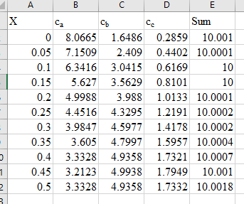
The output is,

ans =

Columns 1 through 5

8.0655 7.1509 6.3416 5.6270 4.9988

Columns 6 through 10

4.4516 3.9847 3.6050 3.3328 3.2123

Column 11

3.3328

Write the all the above equations in matrix form for the reactant B.

$\left[\begin{array}{ccccccccccc}80& -80& 20& 0& 0& 0& 0& 0& 0& 0& 0\\ -50& 81& -30& 0& 0& 0& 0& 0& 0& 0& 0\\ 0& -50& 81& -30& 0& 0& 0& 0& 0& 0& 0\\ 0& 0& -50& 81& -30& 0& 0& 0& 0& 0& 0\\ 0& 0& 0& -50& 81& -30& 0& 0& 0& 0& 0\\ 0& 0& 0& 0& -50& 81& -30& 0& 0& 0& 0\\ 0& 0& 0& 0& 0& -50& 81& -30& 0& 0& 0\\ 0& 0& 0& 0& 0& 0& -50& 81& -30& 0& 0\\ 0& 0& 0& 0& 0& 0& 0& -50& 81& -30& 0\\ 0& 0& 0& 0& 0& 0& 0& 0& -50& 81& -30\\ 0& 0& 0& 0& 0& 0& 0& 0& 0& 81& -80\end{array}\right]\left[\begin{array}{c}{c}_{b,1}\\ c_{b,2}\\ c_{b,3}\\ c_{b,4}\\ c_{b,5}\\ c_{b,6}\\ c_{b,7}\\ c_{b,8}\\ c_{b,9}\\ c_{b,10}\\ c_{b,11}\end{array}\right]=\left[\begin{array}{c}0\\ 21.4527\\ 19.0248\\ 16.8810\\ 14.9964\\ 13.3548\\ 11.9541\\ 10.8150\\ 9.9984\\ 9.6369\\ 9.6369\end{array}\right]$

Write the following code in MATLAB.

A=[80 -80 20 0 0 0 0 0 0 0 0

-50 81 -30 0 0 0 0 0 0 0 0

0 -50 81 -30 0 0 0 0 0 0 0

0 0 -50 81 -30 0 0 0 0 0 0

0 0 0 -50 81 -30 0 0 0 0 0

0 0 0 0 -50 81 -30 0 0 0 0

0 0 0 0 0 -50 81 -30 0 0 0

0 0 0 0 0 0 -50 81 -30 0 0

0 0 0 0 0 0 0 -50 81 -30 0

0 0 0 0 0 0 0 0 -50 81 -30

0 0 0 0 0 0 0 0 0 81 -80];

b=[0;21.4527;19.0248;16.881;14.9964;13.3548;

11.9541;10.815;9.9984;9.6369;9.6369];

c=A\b;

c'

The output is,

ans =

1.6486 2.4090 3.0415 3.5629 3.9880 4.3295 4.5977 4.7997 4.9358

4.9938 4.9358

Write the all the above equations in matrix form for the reactant C.

$\left[\begin{array}{ccccccccccc}80& -80& 20& 0& 0& 0& 0& 0& 0& 0& 0\\ -50& 80& -30& 0& 0& 0& 0& 0& 0& 0& 0\\ 0& -50& 80& -30& 0& 0& 0& 0& 0& 0& 0\\ 0& 0& -50& 80& -30& 0& 0& 0& 0& 0& 0\\ 0& 0& 0& -50& 80& -30& 0& 0& 0& 0& 0\\ 0& 0& 0& 0& -50& 80& -30& 0& 0& 0& 0\\ 0& 0& 0& 0& 0& -50& 80& -30& 0& 0& 0\\ 0& 0& 0& 0& 0& 0& -50& 80& -30& 0& 0\\ 0& 0& 0& 0& 0& 0& 0& -50& 80& -30& 0\\ 0& 0& 0& 0& 0& 0& 0& 0& -50& 80& -30\\ 0& 0& 0& 0& 0& 0& 0& 0& 0& 80& -80\end{array}\right]\left[\begin{array}{c}{c}_{c,1}\\ c_{c,2}\\ c_{c,3}\\ c_{c,4}\\ c_{c,5}\\ c_{c,6}\\ c_{c,7}\\ c_{c,8}\\ c_{c,9}\\ c_{c,10}\\ c_{c,11}\end{array}\right]=\left[\begin{array}{c}0\\ 2.4090\\ 3.0415\\ 3.5629\\ 3.9880\\ 4.3295\\ 4.5977\\ 4.7997\\ 4.9358\\ 4.9938\\ 4.9358\end{array}\right]$

Write the following code in MATLAB.

A=[80 -80 20 0 0 0 0 0 0 0 0

-50 80 -30 0 0 0 0 0 0 0 0

0 -50 80 -30 0 0 0 0 0 0 0

0 0 -50 80 -30 0 0 0 0 0 0

0 0 0 -50 80 -30 0 0 0 0 0

0 0 0 0 -50 80 -30 0 0 0 0

0 0 0 0 0 -50 80 -30 0 0 0

0 0 0 0 0 0 -50 80 -30 0 0

0 0 0 0 0 0 0 -50 80 -30 0

0 0 0 0 0 0 0 0 -50 80 -30

0 0 0 0 0 0 0 0 0 80 -80];

b=[0;2.4090;3.0415;3.5629;3.9880;4.3295;

4.5977;4.7997;4.9358;4.9938;4.9358];

c=A\b;

c'

The output is,

Columns 1 through 7

0.2859 0.4402 0.6169 0.8101 1.0133 1.2191 1.4178

Columns 8 through 11

1.5957 1.7321 1.7949 1.7332

The reaction is in series, thus the system for each reactant is,

The below plot shows the distance versus reactant.