Chapter 2.5, Problem 2.34E

a.

To determine

To find:The relative frequency histogram for the data.

Answer to Problem 2.34E

The relative frequency histogram for the datais shown in Figure-1.

Explanation of Solution

Given information: The data is,

Washington	0	Van Buren	4	Buchanan	0
Adams	5	W.H. Harrison	10	Lincoln	4
Jefferson	6	Tyler*	15	A. Johnson	5
Madison	0	Polk	0	Grant	4
Monroe	2	Taylor	6	Hayes	8
JO. Adams	4	Fillmore*	2	Garfield	7
Jackson	0	Pierce	3	Arthur	3
Cleveland	5	Coolidge	2	Nixon	2
B. Harrison*	3	Hoover	2	Ford	4
McKinley	2	F.D.Roosevelt	6	Carter	4
T. Roosevelt*	6	Truman	1	Reagan*	4
Taft	3	Eisenhower	2	G.H.W. Bush	6
Wilson*	3	Kennedy	3	Clinton	1
Harding	0	L.B.Johmson	2	G.W. Bush	2
				Obama	2

Calculation:

The histogram is shown below.

  

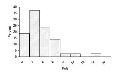
Figure-1

Thus, the relative frequency histogram for the data is shown in Figure-1.

b.

To determine

To find: The mean and standard deviation.

Answer to Problem 2.34E

The mean and standard deviation is $3.5582$ and $2.9139$ .

Explanation of Solution

Given information: The data is,

Washington	0	Van Buren	4	Buchanan	0
Adams	5	W.H. Harrison	10	Lincoln	4
Jefferson	6	Tyler*	15	A. Johnson	5
Madison	0	Polk	0	Grant	4
Monroe	2	Taylor	6	Hayes	8
JO. Adams	4	Fillmore*	2	Garfield	7
Jackson	0	Pierce	3	Arthur	3
Cleveland	5	Coolidge	2	Nixon	2
B. Harrison*	3	Hoover	2	Ford	4
McKinley	2	F.D.Roosevelt	6	Carter	4
T. Roosevelt*	6	Truman	1	Reagan*	4
Taft	3	Eisenhower	2	G.H.W. Bush	6
Wilson*	3	Kennedy	3	Clinton	1
Harding	0	L.B.Johmson	2	G.W. Bush	2
				Obama	2

Calculation:

The mean is,

  $\begin{array}{c}\overline{x}=\frac{{\displaystyle \sum x}}{n}\\ =\frac{153}{43}\\ =3.5582\end{array}$

The variance is,

  $\begin{array}{c}{s}^2=\frac{1}{n-1}\left[{\displaystyle \sum x_i^2}-\frac{{\left({\displaystyle \sum x}\right)}^2}{n}\right]\\ =\frac{1}{43-1}\left[901-\frac{{\left(153\right)}^2}{43}\right]\\ =8.4906\end{array}$

The standard deviation is,

  $\begin{array}{c}s=\sqrt{8.4906}\\ =2.9139\end{array}$

Thus, the mean and standard deviation is $3.5582$ and $2.9139$ .

c.

To determine

To find: The percentage falling into the given intervals.

Answer to Problem 2.34E

The percentage falling into the given intervalsis $95\%$ and $99.7\%$ .

Explanation of Solution

Given information: The data is,

Washington	0	Van Buren	4	Buchanan	0
Adams	5	W.H. Harrison	10	Lincoln	4
Jefferson	6	Tyler*	15	A. Johnson	5
Madison	0	Polk	0	Grant	4
Monroe	2	Taylor	6	Hayes	8
JO. Adams	4	Fillmore*	2	Garfield	7
Jackson	0	Pierce	3	Arthur	3
Cleveland	5	Coolidge	2	Nixon	2
B. Harrison*	3	Hoover	2	Ford	4
McKinley	2	F.D.Roosevelt	6	Carter	4
T. Roosevelt*	6	Truman	1	Reagan*	4
Taft	3	Eisenhower	2	G.H.W. Bush	6
Wilson*	3	Kennedy	3	Clinton	1
Harding	0	L.B.Johmson	2	G.W. Bush	2
				Obama	2

Calculation:

The interval is,

  $\begin{array}{c}\left(\overline{x}\pm s\right)=3.5582\pm 2.9139\\ =\left(0.6443,6.4721\right)\end{array}$

The measurement falling into the intervals are 33.

The interval is,

  $\begin{array}{c}\left(\overline{x}\pm 2s\right)=3.5582\pm 2\times 2.9139\\ =\left(-2.2696,9.386\right)\end{array}$

The measurement falling into the intervals are 41.

The interval is,

  $\begin{array}{c}\left(\overline{x}\pm 3s\right)=3.5582\pm 3\times 2.9139\\ =\left(-5.1835,12.2999\right)\end{array}$

The measurement falling into the intervals are 42.

According to the Empirical formula the percentage of values falling into the intervals are $95\%$ and $99.7\%$

Thus, the percentage falling into the given intervals is $95\%$ and $99.7\%$ .