Concept explainers
To explain and illustrate:
The policy tools that
Concept introduction:
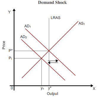
Aggregate Demand Shock: A sudden and large change in the aggregate demand in the economy. This may be due to changes in the expectations about future income or employment trends; changes in the expectations about future inflation or deflation; shift in the structure of demand from domestic economy to foreign country or vice versa; and malfunctioning of financial sector.
Temporary Supply Shock: A supply shock is a sudden increase or decrease in the supply of goods and services in the economy leading to a sudden effect on the economy’s general price level. If due to the supply shock, there is no shift in the long-run
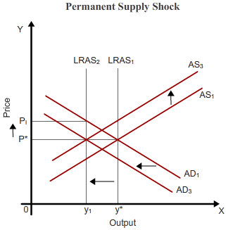
Permanent Supply Shock: If due to the supply shock the long-run aggregate supply curve shifts, then the supply shock is permanent.
Explanation of Solution
The long-run equilibrium income is at Y* with price level P*. As a result of the demand shock, the aggregate demand curve shifts leftward from AD1 to AD2. The economy is in equilibrium at a lower income level Y1 and lower price level P1. There exists a large excess capacity of Y1Y*. In this situation, there is a question whether the government should do anything or not. If the shock is small, then there is no need of policy response. The economy will adjust and will move towards long-run equilibrium. But if the shock is large then the policy makers can adopt counter-cyclical fiscal and monetary policies to deal with the condition. The government can start spending more; the monetary policy can become expansionary which in turn will lower the interest rate to stimulate the economy. The expansionary monetary policy will push the aggregate demand curve back to its initial position, thereby restoring the long-run equilibrium output. The adjustment is shown in the diagram below.
When there is a temporary supply shock, the policymakers encounter a trade-off between stabilizing inflation and enhancing economic activities. They can come up with three policy responses:
- No response
- Policy to stabilize the inflation in the short-run
- Policy to stabilize the economic activity in the short-run.
In case of permanent supply shock, the policymakers can either choose not to respond or initiate policies to stabilize inflation.
A permanent supply shock shifts the long-run aggregate supply curve to the left from LRAS1 to LRAS2 resulting in a fall in
Want to see more full solutions like this?
Chapter 24 Solutions
EBK THE ECONOMICS OF MONEY, BANKING AND


- C. Regression Discontinuity Birth weight is used as a common sign for a newborn's health. In the United States, if a baby has a birthweight below 1500 grams, the newborn is classified as having “very low birth weight". Suppose you want to study the effect of having very low birth weight on the number of hospital visits made before the baby's first birthday. You decide to use Regression Discontinuity to answer this question. The graph below shows the RD model: Number of hospital visits made before baby's first birthday 5 1400 1450 1500 1550 1600 Birthweight (in grams) a. What is the running variable? (5 points) b. What is the cutoff? (5 points) T What is the discontinuity in the graph and how do you interpret it? (10 points)arrow_forwardExperiments Research suggests that if students use laptops in class, it can have some effect on student achievement. While laptop usage can help students take lecture notes faster, some argue that the laptops may be a source of distraction for the students. Suppose you are interested in looking at the effect of using laptops in class on the students' final exam scores out of 100. You decide to conduct a randomized control trial where you randomly assign some students at UIC to use a laptop in class and other to not use a laptop in class. (Assume that the classes are in person and not online) a. Which people are a part of the treatment group and which people are a part of the control group? (10 points) b. What regression will you run? Define the variables where required. (10 points)arrow_forwardExperiments Research suggests that if students use laptops in class, it can have some effect on student achievement. While laptop usage can help students take lecture notes faster, some argue that the laptops may be a source of distraction for the students. Suppose you are interested in looking at the effect of using laptops in class on the students' final exam scores out of 100. You decide to conduct a randomized control trial where you randomly assign some students at UIC to use a laptop in class and other to not use a laptop in class. (Assume that the classes are in person and not online) a. Which people are a part of the treatment group and which people are a part of the control group? (10 points) b. What regression will you run? Define the variables where required. (10 points)arrow_forward
- Dummy variables News reports claim that in the last year television watching has increased. You believe that rising unemployment during Covid may be one of the causes for this. Suppose you are interested in looking at the effect of being unemployed on the hours spent watching Netflix per day. You collect data on 10,000 people from Chicago who are between the age of 20 and 60. You define the dummy variable Unemployed which takes the value 1 for those who are unemployed and 0 for those who are employed. Equation 1: Hours spent watching Netflix₁ = ßo + B₁Unemployed; + ε¿ Following is the output for equation 1: reg hours spent_watching_netflix unemployed Source SS df MS Number of obs 10,000 F(1, 9998) = 14314.03 Model Residual 3539.70065 2472.39364 9,998 1 3539.70065 .247288822 Prob F R-squared == 0.0000 = 0.5888 Total 6012.09429 9,999 . 601269556 Adj R-squared Root MSE = 0.5887 .49728 hours spen~x Coef. Std. Err. t P>|t| [95% Conf. Interval] unemployed cons 1.189908 .0099456 119.64…arrow_forwardDummy variables News reports claim that in the last year television watching has increased. You believe that rising unemployment during Covid may be one of the causes for this. Suppose you are interested in looking at the effect of being unemployed on the hours spent watching Netflix per day. You collect data on 10,000 people from Chicago who are between the age of 20 and 60. You define the dummy variable Unemployed which takes the value 1 for those who are unemployed and 0 for those who are employed. Equation 1: Hours spent watching Netflix₁ = ßo + B₁Unemployed; + ε¿ Following is the output for equation 1: reg hours spent_watching_netflix unemployed Source SS df MS Number of obs 10,000 F(1, 9998) = 14314.03 Model Residual 3539.70065 2472.39364 9,998 1 3539.70065 .247288822 Prob F R-squared == 0.0000 = 0.5888 Total 6012.09429 9,999 . 601269556 Adj R-squared Root MSE = 0.5887 .49728 hours spen~x Coef. Std. Err. t P>|t| [95% Conf. Interval] unemployed cons 1.189908 .0099456 119.64…arrow_forward17. The South African government's distributive stance is clear given its prioritisation of social spending, which includes grants and subsidised goods. Discuss the advantages and disadvantages of an in-kind subsidy versus a cash grant. Use a graphical illustration to support your arguments. [15] 18. Redistributive expenditure can take the form of direct cash transfers (grants) and/or in-kind subsidies. With references to the graphs below, discuss the merits of these two transfer types in the presence and absence of a positive externality. [14] 19. Expenditure on education and healthcare have, by far, the biggest redistributive effect in South Africa' by one estimate dropping the Gini-coefficient by 10 percentage points. Discuss the South African government's performance in health and education provision by evaluating both the outputs and outcomes in these areas of service delivery. [15] 20. Define the following concepts and provide an example in each case: tax rate structure, general…arrow_forward
- Summarise the case for government intervention in the education marketarrow_forwardShould Maureen question the family about the history of the home? Can Maureen access public records for proof of repairs?arrow_forward3. Distinguish between a direct democracy and a representative democracy. Use appropriate examples to support your answers. [4] 4. Explain the distinction between outputs and outcomes in social service delivery [2] 5. A R1000 tax payable by all adults could be viewed as both a proportional tax and a regressive tax. Do you agree? Explain. [4] 6. Briefly explain the displacement effect in Peacock and Wiseman's model of government expenditure growth and provide a relevant example of it in the South African context. [5] 7. Explain how unbalanced productivity growth may affect government expenditure and briefly comment on its relevance to South Africa. [5] 8. South Africa has recently proposed an increase in its value-added tax rate to 15%, sparking much controversy. Why is it argued that value-added tax is inequitable and what can be done to correct the inequity? [5] 9. Briefly explain the difference between access to education and the quality of education, and why we should care about the…arrow_forward
- 20. Factors 01 pro B. the technological innovations available to companies. A. the laws that regulate manufacturers. C. the resources used to create output D. the waste left over after goods are produced. 21. Table 1.1 shows the tradeoff between different combinations of missile production and home construction, ceteris paribus. Complete the table by calculating the required opportunity costs for both missiles and houses. Then answer the indicated question(s). Combination Number of houses Opportunity cost of houses in Number of missiles terms of missiles J 0 4 K 10,000 3 L 17,000 2 1 M 21,000 0 N 23,000 Opportunity cost of missiles in terms of houses Tutorials-Principles of Economics m health carearrow_forwardIn a small open economy with a floating exchange rate, the supply of real money balances is fixed and a rise in government spending ______ Group of answer choices Raises the interest rate so that net exports must fall to maintain equilibrium in the goods market. Cannot change the interest rate so that net exports must fall to maintain equilibrium in the goods market. Cannot change the interest rate so income must rise to maintain equilibrium in the money market Raises the interest rate, so that income must rise to maintain equilibrium in the money market.arrow_forwardSuppose a country with a fixed exchange rate decides to implement a devaluation of its currency and commits to maintaining the new fixed parity. This implies (A) ______________ in the demand for its goods and a monetary (B) _______________. Group of answer choices (A) expansion ; (B) contraction (A) contraction ; (B) expansion (A) expansion ; (B) expansion (A) contraction ; (B) contractionarrow_forward

 Principles of Economics (12th Edition)EconomicsISBN:9780134078779Author:Karl E. Case, Ray C. Fair, Sharon E. OsterPublisher:PEARSON
 Engineering Economy (17th Edition)EconomicsISBN:9780134870069Author:William G. Sullivan, Elin M. Wicks, C. Patrick KoellingPublisher:PEARSON
 Principles of Economics (MindTap Course List)EconomicsISBN:9781305585126Author:N. Gregory MankiwPublisher:Cengage Learning
 Managerial Economics: A Problem Solving ApproachEconomicsISBN:9781337106665Author:Luke M. Froeb, Brian T. McCann, Michael R. Ward, Mike ShorPublisher:Cengage Learning
 Managerial Economics & Business Strategy (Mcgraw-...EconomicsISBN:9781259290619Author:Michael Baye, Jeff PrincePublisher:McGraw-Hill Education