
Concept explainers
Videos
Military spending: The following table presents the amount spent, in billions of dollars, on national defense by the U.S. government every other year for the years 1951 through 2017. The amounts are adjusted for inflation, and represent 2017 dollars.
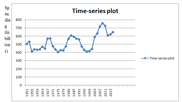
- Construct a time-series plot for these data.
- The plot covers seven decades, from the 1950s through the period 2010—2017. During which of these decades did national defense spending increase, and during which decades did it decrease?
- The United States fought in the Korean War, which ended in 1953. What effect did the end of the war have on military spending after 1953?
- During the period 1965—1963, the United States steadily increased the number of troops in Vietnam from 23,000 at the beginning of 1965 to 537.000 at the end of 1968.
Beginning in 1969, the number of Americans in Vietnam was steadily reduced, with the last of them leaving in 1975. How is this reflected in the national defense spending from 1965 to 1975?
a.
To construct:A time-series plot of the given data.
Explanation of Solution
Given information:
The dataset:
| Year | Spending |
| 1951 | 503.1 |
| 1953 | 531.9 |
| 1955 | 411.9 |
| 1957 | 438.2 |
| 1959 | 432.4 |
| 1961 | 437.6 |
| 1963 | 470.9 |
| 1965 | 447.1 |
| 1967 | 569.3 |
| 1969 | 572.6 |
| 1971 | 476.8 |
| 1973 | 436.9 |
| 1975 | 404.0 |
| 1977 | 427.9 |
| 1979 | 424.4 |
| 1981 | 475.1 |
| 1983 | 568.3 |
| 1985 | 608.3 |
| 1987 | 592.1 |
| 1989 | 568.9 |
| 1991 | 560.1 |
| 1993 | 474.6 |
| 1995 | 429.8 |
| 1997 | 409.8 |
| 1999 | 416.9 |
| 2001 | 442.6 |
| 2003 | 589.0 |
| 2005 | 633.4 |
| 2007 | 718.3 |
| 2009 | 758.4 |
| 2011 | 726.0 |
| 2013 | 608.5 |
| 2015 | 621.2 |
| 2017 | 650.0 |
Graph:
A time-series plot for the given data is given by
b.
To find:The decade during which the national defence spending increasing and the decade during which the national defence spending increasing.
Answer to Problem 27E
The trend in the vacancy rate during the time period from 2012 to 2015 is decreasing.
Explanation of Solution
Solution:
A time-series plot for the given data is given by
From the time-series plot, we can see that during 1960s, 1980s and 2000s, the national defence spending is increasing and during 1950s, 1970s, 1990s and 2010s, the national defence spending is decreasing
Hence,
Increased decade: 1960s, 1980s and 2000s
Decreased decade: 1950s, 1970s, 1990s and 2010s.
c.
To find: The effects of the end of the war have on military spending after 1953.
Answer to Problem 27E
The effects of the end of the war have on military spending after 1953 is that it caught a big decrease.
Explanation of Solution
Solution:
A time-series plot for the given data is given by
From the time-series plot, we can see that after 1953, there was causing a big decrease in the military spending. The military spending was falling from 531.9 to 411.9 during 1953-1955.
Hence, the effects of the end of the war have on military spending after 1953 is that there caused a big decrease.
d.
To explain: The reflection in the national defence spending from 1965 to 1975.
Answer to Problem 27E
The national defence spending is increased from 1965 to 1969 and then decreased from 1969 to 1975.
Explanation of Solution
Given information: The following table presents the amount spent, in billions of dollars, on national defence by the U.S. government every other year for the years 1951 through 2017. The amounts are adjusted for inflation, and represent 2017 dollars.
| Year | Spending |
| 1951 | 503.1 |
| 1953 | 531.9 |
| 1955 | 411.9 |
| 1957 | 438.2 |
| 1959 | 432.4 |
| 1961 | 437.6 |
| 1963 | 470.9 |
| 1965 | 447.1 |
| 1967 | 569.3 |
| 1969 | 572.6 |
| 1971 | 476.8 |
| 1973 | 436.9 |
| 1975 | 404.0 |
| 1977 | 427.9 |
| 1979 | 424.4 |
| 1981 | 475.1 |
| 1983 | 568.3 |
| 1985 | 608.3 |
| 1987 | 592.1 |
| 1989 | 568.9 |
| 1991 | 560.1 |
| 1993 | 474.6 |
| 1995 | 429.8 |
| 1997 | 409.8 |
| 1999 | 416.9 |
| 2001 | 442.6 |
| 2003 | 589.0 |
| 2005 | 633.4 |
| 2007 | 718.3 |
| 2009 | 758.4 |
| 2011 | 726.0 |
| 2013 | 608.5 |
| 2015 | 621.2 |
| 2017 | 650.0 |
During the period 1965-1968, the United States steadily increased the number of troops in Vietnam from 23,000 at the beginning of 1965 to 537,000 at the end of 1968. Beginning in 1969, the number of Americans in Vietnam was steadily reduced, with the last of themleaving in 1975.
A time-series plot for the given data is given by
From 1965 to 1975, the national defence spending is increasing from 1965 to 1969 and then decreasing from 1969 to 1975.
Hence, the national defence spending is increased from 1965 to 1969 and then decreased from 1969 to 1975.
Want to see more full solutions like this?
Chapter 2 Solutions
ELEMENTARY STATISTICS-ALEKS ACCESS CODE


- The acidity or alkalinity of a solution is measured using pH. A pH less than 7 is acidic; a pH greater than 7 is alkaline. The accompanying data represent the pH in samples of bottled water and tap water. Complete parts (a) and (b). Click the icon to view the data table. (a) Determine the mean, median, and mode pH for each type of water. Comment on the differences between the two water types. Select the correct choice below and fill in any answer boxes in your choice. A. For tap water, the mean pH is (Round to three decimal places as needed.) B. The mean does not exist. Data table Тар 7.64 7.45 7.45 7.10 7.46 7.50 7.68 7.69 7.56 7.46 7.52 7.46 5.15 5.09 5.31 5.20 4.78 5.23 Bottled 5.52 5.31 5.13 5.31 5.21 5.24 - ☑arrow_forwardく Chapter 5-Section 1 Homework X MindTap - Cengage Learning x + C webassign.net/web/Student/Assignment-Responses/submit?pos=3&dep=36701632&tags=autosave #question3874894_3 M Gmail 品 YouTube Maps 5. [-/20 Points] DETAILS MY NOTES BBUNDERSTAT12 5.1.020. ☆ B Verify it's you Finish update: All Bookmarks PRACTICE ANOTHER A computer repair shop has two work centers. The first center examines the computer to see what is wrong, and the second center repairs the computer. Let x₁ and x2 be random variables representing the lengths of time in minutes to examine a computer (✗₁) and to repair a computer (x2). Assume x and x, are independent random variables. Long-term history has shown the following times. 01 Examine computer, x₁₁ = 29.6 minutes; σ₁ = 8.1 minutes Repair computer, X2: μ₂ = 92.5 minutes; σ2 = 14.5 minutes (a) Let W = x₁ + x2 be a random variable representing the total time to examine and repair the computer. Compute the mean, variance, and standard deviation of W. (Round your answers…arrow_forwardThe acidity or alkalinity of a solution is measured using pH. A pH less than 7 is acidic; a pH greater than 7 is alkaline. The accompanying data represent the pH in samples of bottled water and tap water. Complete parts (a) and (b). Click the icon to view the data table. (a) Determine the mean, median, and mode pH for each type of water. Comment on the differences between the two water types. Select the correct choice below and fill in any answer boxes in your choice. A. For tap water, the mean pH is (Round to three decimal places as needed.) B. The mean does not exist. Data table Тар Bottled 7.64 7.45 7.46 7.50 7.68 7.45 7.10 7.56 7.46 7.52 5.15 5.09 5.31 5.20 4.78 5.52 5.31 5.13 5.31 5.21 7.69 7.46 5.23 5.24 Print Done - ☑arrow_forward
- The median for the given set of six ordered data values is 29.5. 9 12 23 41 49 What is the missing value? The missing value is ☐.arrow_forwardFind the population mean or sample mean as indicated. Sample: 22, 18, 9, 6, 15 □ Select the correct choice below and fill in the answer box to complete your choice. O A. x= B. μεarrow_forwardWhy the correct answer is letter A? Students in an online course are each randomly assigned to receive either standard practice exercises or adaptivepractice exercises. For the adaptive practice exercises, the next question asked is determined by whether the studentgot the previous question correct. The teacher of the course wants to determine whether there is a differencebetween the two practice exercise types by comparing the proportion of students who pass the course from eachgroup. The teacher plans to test the null hypothesis that versus the alternative hypothesis , whererepresents the proportion of students who would pass the course using standard practice exercises andrepresents the proportion of students who would pass the course using adaptive practice exercises.The teacher knows that the percent confidence interval for the difference in proportion of students passing thecourse for the two practice exercise types (standard minus adaptive) is and the percent…arrow_forward
- Carpetland salespersons average $8,000 per week in sales. Steve Contois, the firm's vice president, proposes a compensation plan with new selling incentives. Steve hopes that the results of a trial selling period will enable him to conclude that the compensation plan increases the average sales per salesperson. a. Develop the appropriate null and alternative hypotheses.H 0: H a:arrow_forwardتوليد تمرين شامل حول الانحدار الخطي المتعدد بطريقة المربعات الصغرىarrow_forwardThe U.S. Postal Service will ship a Priority Mail® Large Flat Rate Box (12" 3 12" 3 5½") any where in the United States for a fixed price, regardless of weight. The weights (ounces) of 20 ran domly chosen boxes are shown below. (a) Make a stem-and-leaf diagram. (b) Make a histogram. (c) Describe the shape of the distribution. Weights 72 86 28 67 64 65 45 86 31 32 39 92 90 91 84 62 80 74 63 86arrow_forward
- (a) What is a bimodal histogram? (b) Explain the difference between left-skewed, symmetric, and right-skewed histograms. (c) What is an outlierarrow_forward(a) Test the hypothesis. Consider the hypothesis test Ho = : against H₁o < 02. Suppose that the sample sizes aren₁ = 7 and n₂ = 13 and that $² = 22.4 and $22 = 28.2. Use α = 0.05. Ho is not ✓ rejected. 9-9 IV (b) Find a 95% confidence interval on of 102. Round your answer to two decimal places (e.g. 98.76).arrow_forwardLet us suppose we have some article reported on a study of potential sources of injury to equine veterinarians conducted at a university veterinary hospital. Forces on the hand were measured for several common activities that veterinarians engage in when examining or treating horses. We will consider the forces on the hands for two tasks, lifting and using ultrasound. Assume that both sample sizes are 6, the sample mean force for lifting was 6.2 pounds with standard deviation 1.5 pounds, and the sample mean force for using ultrasound was 6.4 pounds with standard deviation 0.3 pounds. Assume that the standard deviations are known. Suppose that you wanted to detect a true difference in mean force of 0.25 pounds on the hands for these two activities. Under the null hypothesis, 40 = 0. What level of type II error would you recommend here? Round your answer to four decimal places (e.g. 98.7654). Use a = 0.05. β = i What sample size would be required? Assume the sample sizes are to be equal.…arrow_forward

 College AlgebraAlgebraISBN:9781305115545Author:James Stewart, Lothar Redlin, Saleem WatsonPublisher:Cengage Learning