
Concept explainers
Videos
Ogive: Using the data in Exercise 28:
- Compute the cumulative frequencies for the classes in the American League frequency distribution.
- Construct a frequency ogive for the American League frequency distribution.
- Compute the cumulative relative frequencies for the classes in the American League frequency distribution.
- Construct a relative frequency ogive for the American League, using the same classes.
- Compute the cumulative frequencies for the classes in the National League frequency distribution.
- Construct a frequency ogive for the National League frequency distribution.
- Compute the cumulative relative frequencies for the classes in the National League frequency distribution.
- Construct a relative frequency ogive for the National League, using the same classes.
a.
To compute:The cumulative frequencies for the classes in the American League frequency distribution.
Answer to Problem 44E
| Batting average | American League Cumulative Frequency |
| 0.180-0.199 | 2 |
| 0.200-0.219 | 9 |
| 0.220-0.239 | 30 |
| 0.240-0.259 | 60 |
| 0.260-0.279 | 86 |
| 0.280-0.299 | 107 |
| 0.300-0.319 | 119 |
| 0.320-0.339 | 124 |
| 0.340-0.359 | 124 |
Explanation of Solution
Given information:The following frequency distribution presents the batting averages of Major League Baseball players in both the American League and the National League who had 300 or more plate appearances during a recent season.
| Batting average | American LeagueFrequency | National LeagueFrequency |
| 0.180-0.199 | 2 | 2 |
| 0.200-0.219 | 7 | 7 |
| 0.220-0.239 | 21 | 20 |
| 0.240-0.259 | 30 | 29 |
| 0.260-0.279 | 26 | 32 |
| 0.280-0.299 | 21 | 30 |
| 0.300-0.319 | 12 | 17 |
| 0.320-0.339 | 5 | 5 |
| 0.340-0.359 | 0 | 1 |
Definition used: The cumulative frequency of a class is the sum of the frequencies of that class and all previous classes.
Calculation:
The cumulative classes are given by in the following table.
| Batting average | American LeagueFrequency | American League Cumulative Frequency |
| 0.180-0.199 | 2 | 2 |
| 0.200-0.219 | 7 | |
| 0.220-0.239 | 21 | |
| 0.240-0.259 | 30 | |
| 0.260-0.279 | 26 | |
| 0.280-0.299 | 21 | |
| 0.300-0.319 | 12 | |
| 0.320-0.339 | 5 | |
| 0.340-0.359 | 0 |
Hence, the cumulative frequency for American league is given by
| Batting average | American League Cumulative Frequency |
| 0.180-0.199 | 2 |
| 0.200-0.219 | 9 |
| 0.220-0.239 | 30 |
| 0.240-0.259 | 60 |
| 0.260-0.279 | 86 |
| 0.280-0.299 | 107 |
| 0.300-0.319 | 119 |
| 0.320-0.339 | 124 |
| 0.340-0.359 | 124 |
b.
To find:The frequency ogive for the frequency distribution.
Explanation of Solution
Given information:The following frequency distribution presents the batting averages of Major League Baseball players in both the American League and the National League who had 300 or more plate appearances during a recent season.
| Batting average | American LeagueFrequency | National LeagueFrequency |
| 0.180-0.199 | 2 | 2 |
| 0.200-0.219 | 7 | 7 |
| 0.220-0.239 | 21 | 20 |
| 0.240-0.259 | 30 | 29 |
| 0.260-0.279 | 26 | 32 |
| 0.280-0.299 | 21 | 30 |
| 0.300-0.319 | 12 | 17 |
| 0.320-0.339 | 5 | 5 |
| 0.340-0.359 | 0 | 1 |
Definition used:An ogive plots the cumulative frequencies.
Solution:
The table of cumulative American League frequency is given by
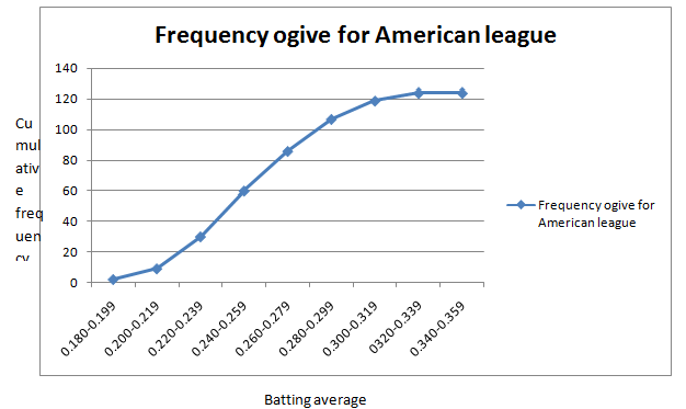
| Batting average | American League Cumulative Frequency |
| 0.180-0.199 | 2 |
| 0.200-0.219 | 9 |
| 0.220-0.239 | 30 |
| 0.240-0.259 | 60 |
| 0.260-0.279 | 86 |
| 0.280-0.299 | 107 |
| 0.300-0.319 | 119 |
| 0.320-0.339 | 124 |
| 0.340-0.359 | 124 |
The frequency ogivefor American League frequency distribution is given by
c.
To compute: The cumulative relative frequencies for the classes in the American league frequency distribution.
Answer to Problem 44E
| Batting average | Cumulative relative Frequency |
| 0.180-0.199 | 0.016 |
| 0.200-0.219 | 0.073 |
| 0.220-0.239 | 0.242 |
| 0.240-0.259 | 0.484 |
| 0.260-0.279 | 0.694 |
| 0.280-0.299 | 0.863 |
| 0.300-0.319 | 0.960 |
| 0.320-0.339 | 1.000 |
| 0.340-0.359 | 1.000 |
Explanation of Solution
Given information: The following frequency distribution presents the batting averages of Major League Baseball players in both the American League and the National League who had 300 or more plate appearances during a recent season.
| Batting average | American LeagueFrequency | National LeagueFrequency |
| 0.180-0.199 | 2 | 2 |
| 0.200-0.219 | 7 | 7 |
| 0.220-0.239 | 21 | 20 |
| 0.240-0.259 | 30 | 29 |
| 0.260-0.279 | 26 | 32 |
| 0.280-0.299 | 21 | 30 |
| 0.300-0.319 | 12 | 17 |
| 0.320-0.339 | 5 | 5 |
| 0.340-0.359 | 0 | 1 |
Definition used: The cumulative relative frequency of a class is given by
Calculation:
The cumulative classes are given by in the following table.
| Batting average | American League Cumulative Frequency | American League relative Cumulative Frequency |
| 0.180-0.199 | 2 | |
| 0.200-0.219 | 9 | |
| 0.220-0.239 | 30 | |
| 0.240-0.259 | 60 | |
| 0.260-0.279 | 86 | |
| 0.280-0.299 | 107 | |
| 0.300-0.319 | 119 | |
| 0.320-0.339 | 124 | |
| 0.340-0.359 | 124 |
Hence, the cumulative relative frequency is given by
| Batting average | Cumulative relative Frequency |
| 0.180-0.199 | 0.016 |
| 0.200-0.219 | 0.073 |
| 0.220-0.239 | 0.242 |
| 0.240-0.259 | 0.484 |
| 0.260-0.279 | 0.694 |
| 0.280-0.299 | 0.863 |
| 0.300-0.319 | 0.960 |
| 0.320-0.339 | 1.000 |
| 0.340-0.359 | 1.000 |
d.
To find: The relative frequency ogive for the American league frequency distribution.
Explanation of Solution
Given information:The following frequency distribution presents the batting averages of Major League Baseball players in both the American League and the National League who had 300 or more plate appearances during a recent season.
| Batting average | American LeagueFrequency | National LeagueFrequency |
| 0.180-0.199 | 2 | 2 |
| 0.200-0.219 | 7 | 7 |
| 0.220-0.239 | 21 | 20 |
| 0.240-0.259 | 30 | 29 |
| 0.260-0.279 | 26 | 32 |
| 0.280-0.299 | 21 | 30 |
| 0.300-0.319 | 12 | 17 |
| 0.320-0.339 | 5 | 5 |
| 0.340-0.359 | 0 | 1 |
Definition used:A relative frequency ogive plots the cumulative relative frequencies..
Solution:
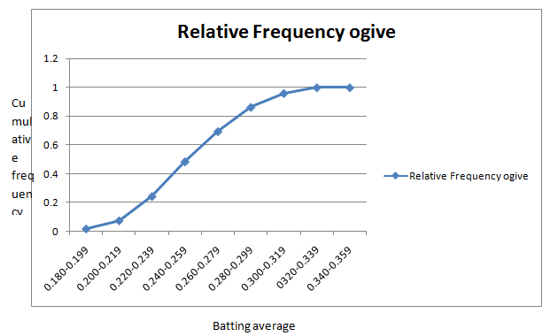
The table of cumulative relative frequency is given by
| Batting average | Cumulative relative Frequency |
| 0.180-0.199 | 0.016 |
| 0.200-0.219 | 0.073 |
| 0.220-0.239 | 0.242 |
| 0.240-0.259 | 0.484 |
| 0.260-0.279 | 0.694 |
| 0.280-0.299 | 0.863 |
| 0.300-0.319 | 0.960 |
| 0.320-0.339 | 1.000 |
| 0.340-0.359 | 1.000 |
The relative frequency ogive is given by
e.
To compute: The cumulative frequencies for the classes in the National League frequency distribution.
Answer to Problem 44E
| Batting average | National League Cumulative Frequency |
| 0.180-0.199 | 2 |
| 0.200-0.219 | 9 |
| 0.220-0.239 | 29 |
| 0.240-0.259 | 58 |
| 0.260-0.279 | 90 |
| 0.280-0.299 | 120 |
| 0.300-0.319 | 137 |
| 0.320-0.339 | 142 |
| 0.340-0.359 | 143 |
Explanation of Solution
Given information: The following frequency distribution presents the batting averages of Major League Baseball players in both the American League and the National League who had 300 or more plate appearances during a recent season.
| Batting average | American LeagueFrequency | National LeagueFrequency |
| 0.180-0.199 | 2 | 2 |
| 0.200-0.219 | 7 | 7 |
| 0.220-0.239 | 21 | 20 |
| 0.240-0.259 | 30 | 29 |
| 0.260-0.279 | 26 | 32 |
| 0.280-0.299 | 21 | 30 |
| 0.300-0.319 | 12 | 17 |
| 0.320-0.339 | 5 | 5 |
| 0.340-0.359 | 0 | 1 |
Definition used: The cumulative frequency of a class is the sum of the frequencies of that class and all previous classes.
Calculation:
The cumulative classes are given by in the following table.
| Batting average | National LeagueFrequency | National League Cumulative Frequency |
| 0.180-0.199 | 2 | 2 |
| 0.200-0.219 | 7 | |
| 0.220-0.239 | 20 | |
| 0.240-0.259 | 29 | |
| 0.260-0.279 | 32 | |
| 0.280-0.299 | 30 | |
| 0.300-0.319 | 17 | |
| 0.320-0.339 | 5 | |
| 0.340-0.359 | 1 |
Hence, the cumulative frequency for National league is given by
| Batting average | National League Cumulative Frequency |
| 0.180-0.199 | 2 |
| 0.200-0.219 | 9 |
| 0.220-0.239 | 29 |
| 0.240-0.259 | 58 |
| 0.260-0.279 | 90 |
| 0.280-0.299 | 120 |
| 0.300-0.319 | 137 |
| 0.320-0.339 | 142 |
| 0.340-0.359 | 143 |
h.
To find: The frequency ogive for the National League frequency distribution.
Explanation of Solution
Given information:The following frequency distribution presents the batting averages of Major League Baseball players in both the American League and the National League who had 300 or more plate appearances during a recent season.
| Batting average | American LeagueFrequency | National LeagueFrequency |
| 0.180-0.199 | 2 | 2 |
| 0.200-0.219 | 7 | 7 |
| 0.220-0.239 | 21 | 20 |
| 0.240-0.259 | 30 | 29 |
| 0.260-0.279 | 26 | 32 |
| 0.280-0.299 | 21 | 30 |
| 0.300-0.319 | 12 | 17 |
| 0.320-0.339 | 5 | 5 |
| 0.340-0.359 | 0 | 1 |
Definition used: An ogive plots the cumulative frequencies.
Solution:
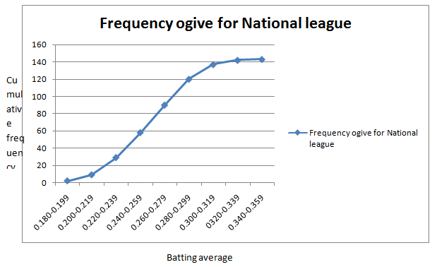
The table of cumulative National League frequency is given by
| Batting average | National League Cumulative Frequency |
| 0.180-0.199 | 2 |
| 0.200-0.219 | 9 |
| 0.220-0.239 | 29 |
| 0.240-0.259 | 58 |
| 0.260-0.279 | 90 |
| 0.280-0.299 | 120 |
| 0.300-0.319 | 137 |
| 0.320-0.339 | 142 |
| 0.340-0.359 | 143 |
The frequency ogive for National League frequency distribution is given by
g.
To compute: The cumulative relative frequencies for the classes in the National league frequency distribution.
Answer to Problem 44E
| Batting average | Cumulative relative Frequency |
| 0.180-0.199 | 0.014 |
| 0.200-0.219 | 0.063 |
| 0.220-0.239 | 0.203 |
| 0.240-0.259 | 0.406 |
| 0.260-0.279 | 0.629 |
| 0.280-0.299 | 0.839 |
| 0.300-0.319 | 0.958 |
| 0.320-0.339 | 0.993 |
| 0.340-0.359 | 1.000 |
Explanation of Solution
Given information: The following frequency distribution presents the batting averages of Major League Baseball players in both the American League and the National League who had 300 or more plate appearances during a recent season.
| Batting average | American LeagueFrequency | National LeagueFrequency |
| 0.180-0.199 | 2 | 2 |
| 0.200-0.219 | 7 | 7 |
| 0.220-0.239 | 21 | 20 |
| 0.240-0.259 | 30 | 29 |
| 0.260-0.279 | 26 | 32 |
| 0.280-0.299 | 21 | 30 |
| 0.300-0.319 | 12 | 17 |
| 0.320-0.339 | 5 | 5 |
| 0.340-0.359 | 0 | 1 |
Definition used: The cumulative relative frequency of a class is given by
Calculation:
The cumulative classes are given by in the following table.
| Batting average | National League Cumulative Frequency | Cumulative relative frequency |
| 0.180-0.199 | 2 | |
| 0.200-0.219 | 9 | |
| 0.220-0.239 | 29 | |
| 0.240-0.259 | 58 | |
| 0.260-0.279 | 90 | |
| 0.280-0.299 | 120 | |
| 0.300-0.319 | 137 | |
| 0.320-0.339 | 142 | |
| 0.340-0.359 | 143 |
Hence, the cumulative relative frequency for National league is given by
| Batting average | Cumulative relative Frequency |
| 0.180-0.199 | 0.014 |
| 0.200-0.219 | 0.063 |
| 0.220-0.239 | 0.203 |
| 0.240-0.259 | 0.406 |
| 0.260-0.279 | 0.629 |
| 0.280-0.299 | 0.839 |
| 0.300-0.319 | 0.958 |
| 0.320-0.339 | 0.993 |
| 0.340-0.359 | 1.000 |
h.
To find: The relative frequency ogive for the National league frequency distribution.
Explanation of Solution
Given information:The following frequency distribution presents the batting averages of Major League Baseball players in both the American League and the National League who had 300 or more plate appearances during a recent season.
| Batting average | American LeagueFrequency | National LeagueFrequency |
| 0.180-0.199 | 2 | 2 |
| 0.200-0.219 | 7 | 7 |
| 0.220-0.239 | 21 | 20 |
| 0.240-0.259 | 30 | 29 |
| 0.260-0.279 | 26 | 32 |
| 0.280-0.299 | 21 | 30 |
| 0.300-0.319 | 12 | 17 |
| 0.320-0.339 | 5 | 5 |
| 0.340-0.359 | 0 | 1 |
Definition used:A relative frequency ogive plots the cumulative relative frequencies..
Solution:
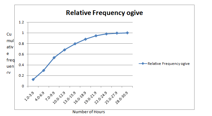
The table of cumulative relative frequency for the National league frequency distribution is given by
| Batting average | Cumulative relative Frequency |
| 0.180-0.199 | 0.014 |
| 0.200-0.219 | 0.063 |
| 0.220-0.239 | 0.203 |
| 0.240-0.259 | 0.406 |
| 0.260-0.279 | 0.629 |
| 0.280-0.299 | 0.839 |
| 0.300-0.319 | 0.958 |
| 0.320-0.339 | 0.993 |
| 0.340-0.359 | 1.000 |
The relative frequency ogivefor National League is given by
Want to see more full solutions like this?
Chapter 2 Solutions
ELEMENTARY STATISTICS W/CONNECT >C<


- Exercise 6-6 (Algo) (LO6-3) The director of admissions at Kinzua University in Nova Scotia estimated the distribution of student admissions for the fall semester on the basis of past experience. Admissions Probability 1,100 0.5 1,400 0.4 1,300 0.1 Click here for the Excel Data File Required: What is the expected number of admissions for the fall semester? Compute the variance and the standard deviation of the number of admissions. Note: Round your standard deviation to 2 decimal places.arrow_forward1. Find the mean of the x-values (x-bar) and the mean of the y-values (y-bar) and write/label each here: 2. Label the second row in the table using proper notation; then, complete the table. In the fifth and sixth columns, show the 'products' of what you're multiplying, as well as the answers. X y x minus x-bar y minus y-bar (x minus x-bar)(y minus y-bar) (x minus x-bar)^2 xy 16 20 34 4-2 5 2 3. Write the sums that represents Sxx and Sxy in the table, at the bottom of their respective columns. 4. Find the slope of the Regression line: bi = (simplify your answer) 5. Find the y-intercept of the Regression line, and then write the equation of the Regression line. Show your work. Then, BOX your final answer. Express your line as "y-hat equals...arrow_forwardApply STATA commands & submit the output for each question only when indicated below i. Generate the log of birthweight and family income of children. Name these new variables Ibwght & Ifaminc. Include the output of this code. ii. Apply the command sum with the detail option to the variable faminc. Note: you should find the 25th percentile value, the 50th percentile and the 75th percentile value of faminc from the output - you will need it to answer the next question Include the output of this code. iii. iv. Use the output from part ii of this question to Generate a variable called "high_faminc" that takes a value 1 if faminc is less than or equal to the 25th percentile, it takes the value 2 if faminc is greater than 25th percentile but less than or equal to the 50th percentile, it takes the value 3 if faminc is greater than 50th percentile but less than or equal to the 75th percentile, it takes the value 4 if faminc is greater than the 75th percentile. Include the outcome of this code…arrow_forward
- solve this on paperarrow_forwardApply STATA commands & submit the output for each question only when indicated below i. Apply the command egen to create a variable called "wyd" which is the rowtotal function on variables bwght & faminc. ii. Apply the list command for the first 10 observations to show that the code in part i worked. Include the outcome of this code iii. Apply the egen command to create a new variable called "bwghtsum" using the sum function on variable bwght by the variable high_faminc (Note: need to apply the bysort' statement) iv. Apply the "by high_faminc" statement to find the V. descriptive statistics of bwght and bwghtsum Include the output of this code. Why is there a difference between the standard deviations of bwght and bwghtsum from part iv of this question?arrow_forwardAccording to a health information website, the distribution of adults’ diastolic blood pressure (in millimeters of mercury, mmHg) can be modeled by a normal distribution with mean 70 mmHg and standard deviation 20 mmHg. b. Above what diastolic pressure would classify someone in the highest 1% of blood pressures? Show all calculations used.arrow_forward
- Write STATA codes which will generate the outcomes in the questions & submit the output for each question only when indicated below i. ii. iii. iv. V. Write a code which will allow STATA to go to your favorite folder to access your files. Load the birthweight1.dta dataset from your favorite folder and save it under a different filename to protect data integrity. Call the new dataset babywt.dta (make sure to use the replace option). Verify that it contains 2,998 observations and 8 variables. Include the output of this code. Are there missing observations for variable(s) for the variables called bwght, faminc, cigs? How would you know? (You may use more than one code to show your answer(s)) Include the output of your code (s). Write the definitions of these variables: bwght, faminc, male, white, motheduc,cigs; which of these variables are categorical? [Hint: use the labels of the variables & the browse command] Who is this dataset about? Who can use this dataset to answer what kind of…arrow_forwardApply STATA commands & submit the output for each question only when indicated below İ. ii. iii. iv. V. Apply the command summarize on variables bwght and faminc. What is the average birthweight of babies and family income of the respondents? Include the output of this code. Apply the tab command on the variable called male. How many of the babies and what share of babies are male? Include the output of this code. Find the summary statistics (i.e. use the sum command) of the variables bwght and faminc if the babies are white. Include the output of this code. Find the summary statistics (i.e. use the sum command) of the variables bwght and faminc if the babies are male but not white. Include the output of this code. Using your answers to previous subparts of this question: What is the difference between the average birthweight of a baby who is male and a baby who is male but not white? What can you say anything about the difference in family income of the babies that are male and male…arrow_forwardA public health researcher is studying the impacts of nudge marketing techniques on shoppers vegetablesarrow_forward
- The director of admissions at Kinzua University in Nova Scotia estimated the distribution of student admissions for the fall semester on the basis of past experience. Admissions Probability 1,100 0.5 1,400 0.4 1,300 0.1 Click here for the Excel Data File Required: What is the expected number of admissions for the fall semester? Compute the variance and the standard deviation of the number of admissions. Note: Round your standard deviation to 2 decimal places.arrow_forwardA pollster randomly selected four of 10 available people. Required: How many different groups of 4 are possible? What is the probability that a person is a member of a group? Note: Round your answer to 3 decimal places.arrow_forwardWind Mountain is an archaeological study area located in southwestern New Mexico. Potsherds are broken pieces of prehistoric Native American clay vessels. One type of painted ceramic vessel is called Mimbres classic black-on-white. At three different sites the number of such sherds was counted in local dwelling excavations. Test given. Site I Site II Site III 63 19 60 43 34 21 23 49 51 48 11 15 16 46 26 20 31 Find .arrow_forward
 Holt Mcdougal Larson Pre-algebra: Student Edition...AlgebraISBN:9780547587776Author:HOLT MCDOUGALPublisher:HOLT MCDOUGAL
 Glencoe Algebra 1, Student Edition, 9780079039897...AlgebraISBN:9780079039897Author:CarterPublisher:McGraw Hill
 Big Ideas Math A Bridge To Success Algebra 1: Stu...AlgebraISBN:9781680331141Author:HOUGHTON MIFFLIN HARCOURTPublisher:Houghton Mifflin Harcourt