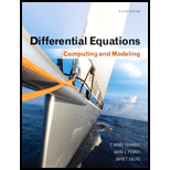
Differential Equations: Computing and Modeling (5th Edition), Edwards, Penney & Calvis
5th Edition
ISBN: 9780321816252
Author: C. Henry Edwards, David E. Penney, David Calvis
Publisher: PEARSON
expand_more
expand_more
format_list_bulleted
Concept explainers
Question
Chapter 2.2, Problem 22P
Program Plan Intro
Program Description: Purpose of problem is to determine the dependence of the number of critical points on the parameter
Expert Solution & Answer
Want to see the full answer?
Check out a sample textbook solution
Students have asked these similar questions
(x)=2x-x2
2
a=2, b = 1/2, C=0
b) Vertex v
F(x)=ax 2 + bx + c
x=
Za
V=2.0L
YEF(- =) = 4
b
(글)
JANUARY 17, 2025
WORKSHEET 1
Solve the following four problems on a separate sheet. Fully justify your answers to
MATH 122
ล
T
earn full credit.
1. Let f(x) = 2x-
1x2
2
(a) Rewrite this quadratic function in standard form: f(x) = ax² + bx + c
and indicate the values of the coefficients: a, b and c.
(b) Find the vertex V, focus F, focal width, directrix D, and the axis of
symmetry for the graph of y = f(x).
(c) Plot a graph of y = f(x) and indicate all quantities found in part (b)
on your graph.
(d) Specify the domain and range of the function f.
OUR
2. Let g(x) = f(x) u(x) where f is the quadratic function from problem 1
and u is the unit step function:
u(x) = { 0
1 if x ≥0
0 if x<0
y = u(x)
0
(a) Write a piecewise formula for the function g.
(b) Sketch a graph of y = g(x).
(c) Indicate the domain and range of the function g.
X
фирм
where u is the unit step function defined in problem 2.
3. Let…
"P3
Question 3: Construct the accessibility matrix Passociated with
the following graphs, and compute P2 and identify each at the
various two-step paths in the graph
Ps
P₁
P₂
A cable television company estimates that with x thousand subscribers, its monthly revenue and cost (in thousands of dollars) are given by the following equations.
R(x) = 45x - 0.24x2 C(x) = 257 + 13x
Chapter 2 Solutions
Differential Equations: Computing and Modeling (5th Edition), Edwards, Penney & Calvis
Ch. 2.1 - Prob. 1PCh. 2.1 - Prob. 2PCh. 2.1 - Prob. 3PCh. 2.1 - Prob. 4PCh. 2.1 - Prob. 5PCh. 2.1 - Prob. 6PCh. 2.1 - Prob. 7PCh. 2.1 - Prob. 8PCh. 2.1 - Prob. 9PCh. 2.1 - Prob. 10P
Ch. 2.1 - Prob. 11PCh. 2.1 - Prob. 12PCh. 2.1 - Prob. 13PCh. 2.1 - Prob. 14PCh. 2.1 - Prob. 15PCh. 2.1 - Prob. 16PCh. 2.1 - Prob. 17PCh. 2.1 - Prob. 18PCh. 2.1 - Prob. 19PCh. 2.1 - Prob. 20PCh. 2.1 - Prob. 21PCh. 2.1 - Suppose that at time t=0, half of a logistic...Ch. 2.1 - Prob. 23PCh. 2.1 - Prob. 24PCh. 2.1 - Prob. 25PCh. 2.1 - Prob. 26PCh. 2.1 - Prob. 27PCh. 2.1 - Prob. 28PCh. 2.1 - Prob. 29PCh. 2.1 - A tumor may be regarded as a population of...Ch. 2.1 - Prob. 31PCh. 2.1 - Prob. 32PCh. 2.1 - Prob. 33PCh. 2.1 - Prob. 34PCh. 2.1 - Prob. 35PCh. 2.1 - Prob. 36PCh. 2.1 - Prob. 37PCh. 2.1 - Fit the logistic equation to the actual U.S....Ch. 2.1 - Prob. 39PCh. 2.2 - Prob. 1PCh. 2.2 - Prob. 2PCh. 2.2 - Prob. 3PCh. 2.2 - Prob. 4PCh. 2.2 - Prob. 5PCh. 2.2 - Prob. 6PCh. 2.2 - Prob. 7PCh. 2.2 - Prob. 8PCh. 2.2 - Prob. 9PCh. 2.2 - Prob. 10PCh. 2.2 - Prob. 11PCh. 2.2 - Prob. 12PCh. 2.2 - Prob. 13PCh. 2.2 - Prob. 14PCh. 2.2 - Prob. 15PCh. 2.2 - Prob. 16PCh. 2.2 - Prob. 17PCh. 2.2 - Prob. 18PCh. 2.2 - Prob. 19PCh. 2.2 - Prob. 20PCh. 2.2 - Prob. 21PCh. 2.2 - Prob. 22PCh. 2.2 - Prob. 23PCh. 2.2 - Prob. 24PCh. 2.2 - Use the alternatives forms...Ch. 2.2 - Prob. 26PCh. 2.2 - Prob. 27PCh. 2.2 - Prob. 28PCh. 2.2 - Consider the two differentiable equation...Ch. 2.3 - The acceleration of a Maserati is proportional to...Ch. 2.3 - Prob. 2PCh. 2.3 - Prob. 3PCh. 2.3 - Prob. 4PCh. 2.3 - Prob. 5PCh. 2.3 - Prob. 6PCh. 2.3 - Prob. 7PCh. 2.3 - Prob. 8PCh. 2.3 - A motorboat weighs 32,000 lb and its motor...Ch. 2.3 - A woman bails out of an airplane at an altitude of...Ch. 2.3 - According to a newspaper account, a paratrooper...Ch. 2.3 - Prob. 12PCh. 2.3 - Prob. 13PCh. 2.3 - Prob. 14PCh. 2.3 - Prob. 15PCh. 2.3 - Prob. 16PCh. 2.3 - Prob. 17PCh. 2.3 - Prob. 18PCh. 2.3 - Prob. 19PCh. 2.3 - Prob. 20PCh. 2.3 - Prob. 21PCh. 2.3 - Suppose that =0.075 (in fps units, with g=32ft/s2...Ch. 2.3 - Prob. 23PCh. 2.3 - The mass of the sun is 329,320 times that of the...Ch. 2.3 - Prob. 25PCh. 2.3 - Suppose that you are stranded—your rocket engine...Ch. 2.3 - Prob. 27PCh. 2.3 - (a) Suppose that a body is dropped (0=0) from a...Ch. 2.3 - Prob. 29PCh. 2.3 - Prob. 30PCh. 2.4 - Prob. 1PCh. 2.4 - Prob. 2PCh. 2.4 - Prob. 3PCh. 2.4 - Prob. 4PCh. 2.4 - Prob. 5PCh. 2.4 - Prob. 6PCh. 2.4 - Prob. 7PCh. 2.4 - Prob. 8PCh. 2.4 - Prob. 9PCh. 2.4 - Prob. 10PCh. 2.4 - Prob. 11PCh. 2.4 - Prob. 12PCh. 2.4 - Prob. 13PCh. 2.4 - Prob. 14PCh. 2.4 - Prob. 15PCh. 2.4 - Prob. 16PCh. 2.4 - Prob. 17PCh. 2.4 - Prob. 18PCh. 2.4 - Prob. 19PCh. 2.4 - Prob. 20PCh. 2.4 - Prob. 21PCh. 2.4 - Prob. 22PCh. 2.4 - Prob. 23PCh. 2.4 - Prob. 24PCh. 2.4 - Prob. 25PCh. 2.4 - Prob. 26PCh. 2.4 - Prob. 27PCh. 2.4 - Prob. 28PCh. 2.4 - Prob. 29PCh. 2.4 - Prob. 30PCh. 2.4 - Prob. 31PCh. 2.5 - Prob. 1PCh. 2.5 - Prob. 2PCh. 2.5 - Prob. 3PCh. 2.5 - Prob. 4PCh. 2.5 - Prob. 5PCh. 2.5 - Prob. 6PCh. 2.5 - Prob. 7PCh. 2.5 - Prob. 8PCh. 2.5 - Prob. 9PCh. 2.5 - Prob. 10PCh. 2.5 - Prob. 11PCh. 2.5 - Prob. 12PCh. 2.5 - Prob. 13PCh. 2.5 - Prob. 14PCh. 2.5 - Prob. 15PCh. 2.5 - Prob. 16PCh. 2.5 - Prob. 17PCh. 2.5 - Prob. 18PCh. 2.5 - Prob. 19PCh. 2.5 - Prob. 20PCh. 2.5 - Prob. 21PCh. 2.5 - Prob. 22PCh. 2.5 - Prob. 23PCh. 2.5 - Prob. 24PCh. 2.5 - Prob. 25PCh. 2.5 - Prob. 26PCh. 2.5 - Prob. 27PCh. 2.5 - Prob. 28PCh. 2.5 - Prob. 29PCh. 2.5 - Prob. 30PCh. 2.6 - Prob. 1PCh. 2.6 - Prob. 2PCh. 2.6 - Prob. 3PCh. 2.6 - Prob. 4PCh. 2.6 - Prob. 5PCh. 2.6 - Prob. 6PCh. 2.6 - Prob. 7PCh. 2.6 - Prob. 8PCh. 2.6 - Prob. 9PCh. 2.6 - Prob. 10PCh. 2.6 - Prob. 11PCh. 2.6 - Prob. 12PCh. 2.6 - Prob. 13PCh. 2.6 - Prob. 14PCh. 2.6 - Prob. 15PCh. 2.6 - Prob. 16PCh. 2.6 - Prob. 17PCh. 2.6 - Prob. 18PCh. 2.6 - Prob. 19PCh. 2.6 - Prob. 20PCh. 2.6 - Prob. 21PCh. 2.6 - Prob. 22PCh. 2.6 - Prob. 23PCh. 2.6 - Prob. 24PCh. 2.6 - Prob. 25PCh. 2.6 - Prob. 26PCh. 2.6 - Prob. 27PCh. 2.6 - Prob. 28PCh. 2.6 - Prob. 29PCh. 2.6 - Prob. 30P
Knowledge Booster
Learn more about
Need a deep-dive on the concept behind this application? Look no further. Learn more about this topic, computer-science and related others by exploring similar questions and additional content below.Similar questions
- x³-343 If k(x) = x-7 complete the table and use the results to find lim k(x). X-7 x 6.9 6.99 6.999 7.001 7.01 7.1 k(x) Complete the table. X 6.9 6.99 6.999 7.001 7.01 7.1 k(x) (Round to three decimal places as needed.)arrow_forward(3) (4 points) Given three vectors a, b, and c, suppose: |bx c = 2 |a|=√√8 • The angle between a and b xc is 0 = 135º. . Calculate the volume a (bxc) of the parallelepiped spanned by the three vectors.arrow_forwardCalculate these limits. If the limit is ∞ or -∞, write infinity or-infinity. If the limit does not exist, write DNE: Hint: Remember the first thing you check when you are looking at a limit of a quotient is the limit value of the denominator. 1. If the denominator does not go to 0, you should be able to right down the answer immediately. 2. If the denominator goes to 0, but the numerator does not, you will have to check the sign (±) of the quotient, from both sides if the limit is not one-sided. 3. If both the numerator and the denominator go to 0, you have to do the algebraic trick of rationalizing. So, group your limits into these three forms and work with them one group at a time. (a) lim t-pi/2 sint-√ sin 2t+14cos ² t 7 2 2 2cos t (b) lim sint + sin 2t+14cos = ∞ t-pi/2 2 2cos t (c) lim cost-√sin 2t+14cos² t = t-pi/2 2cos t (d) lim t→pi/2 cost+√ sin t + 14cos 2cos ² t = ∞ (e) lim sint-v sin 2 t + 14cos = 0 t-pi/2 (f) lim t-pi/2 sin t +√ sin 2sin 2 t 2 t + 14cos t 2sin t cost- (g)…arrow_forward
- Think of this sheet of paper as the plane containing the vectors a = (1,1,0) and b = (2,0,0). Sketch the parallelogram P spanned by a and b. Which diagonal of P represents the vector a--b geometrically?arrow_forward(1) (14 points) Let a = (-2, 10, -4) and b = (3, 1, 1). (a) (4 points) Using the dot product determine the angle between a and b. (b) (2 points) Determine the cross product vector axb. (c) (4 points) Calculate the area of the parallelogram spanned by a and b. Justify your answer. 1arrow_forward(d) (4 points) Think of this sheet of paper as the plane containing the vectors a = (1,1,0) and b = (2,0,0). Sketch the parallelogram P spanned by a and b. Which diagonal of P represents the vector ab geometrically? d be .dx adjarrow_forward
- (2) (4 points) Find all vectors v having length 1 that are perpendicular to both =(2,0,2) and j = (0,1,0). Show all work. a=arrow_forwardFor the following function, find the full power series centered at a of convergence. 0 and then give the first 5 nonzero terms of the power series and the open interval = f(2) Σ 8 1(x)--(-1)*(3)* n=0 ₤(x) = + + + ++... The open interval of convergence is: 1 1 3 f(x)= = 28 3x6 +1 (Give your answer in help (intervals) .)arrow_forwardFor the following function, find the full power series centered at x = 0 and then give the first 5 nonzero terms of the power series and the open interval of convergence. f(x) = Σ| n=0 9 f(x) = 6 + 4x f(x)− + + + ++··· The open interval of convergence is: ☐ (Give your answer in help (intervals) .)arrow_forward
- Let X be a random variable with the standard normal distribution, i.e.,X has the probability density functionfX(x) = 1/√2π e^-(x^2/2)2 .Consider the random variablesXn = 20(3 + X6) ^1/2n e ^x^2/n+19 , x ∈ R, n ∈ N.Using the dominated convergence theorem, prove that the limit exists and find it limn→∞E(Xn)arrow_forwardLet X be a discrete random variable taking values in {0, 1, 2, . . . }with the probability generating function G(s) = E(sX). Prove thatVar(X) = G′′(1) + G′(1) − [G′(1)]2.[5 Marks](ii) Let X be a random variable taking values in [0,∞) with proba-bility density functionfX(u) = (5/4(1 − u^4, 0 ≤ u ≤ 1,0, otherwise. Let y =x^1/2 find the probability density function of Yarrow_forward2. y 1 Ο 2 3 4 -1 Graph of f x+ The graph gives one cycle of a periodic function f in the xy-plane. Which of the following describes the behavior of f on the interval 39 x < 41 ? (Α B The function f is decreasing. The function f is increasing. The function f is decreasing, then increasing. D The function f is increasing, then decreasing.arrow_forward
arrow_back_ios
SEE MORE QUESTIONS
arrow_forward_ios
Recommended textbooks for you
 Calculus: Early TranscendentalsCalculusISBN:9781285741550Author:James StewartPublisher:Cengage Learning
 Thomas' Calculus (14th Edition)CalculusISBN:9780134438986Author:Joel R. Hass, Christopher E. Heil, Maurice D. WeirPublisher:PEARSON
 Calculus: Early Transcendentals (3rd Edition)CalculusISBN:9780134763644Author:William L. Briggs, Lyle Cochran, Bernard Gillett, Eric SchulzPublisher:PEARSON
 Calculus: Early TranscendentalsCalculusISBN:9781319050740Author:Jon Rogawski, Colin Adams, Robert FranzosaPublisher:W. H. Freeman
 Calculus: Early Transcendental FunctionsCalculusISBN:9781337552516Author:Ron Larson, Bruce H. EdwardsPublisher:Cengage Learning

Calculus: Early Transcendentals
Calculus
ISBN:9781285741550
Author:James Stewart
Publisher:Cengage Learning

Thomas' Calculus (14th Edition)
Calculus
ISBN:9780134438986
Author:Joel R. Hass, Christopher E. Heil, Maurice D. Weir
Publisher:PEARSON

Calculus: Early Transcendentals (3rd Edition)
Calculus
ISBN:9780134763644
Author:William L. Briggs, Lyle Cochran, Bernard Gillett, Eric Schulz
Publisher:PEARSON

Calculus: Early Transcendentals
Calculus
ISBN:9781319050740
Author:Jon Rogawski, Colin Adams, Robert Franzosa
Publisher:W. H. Freeman


Calculus: Early Transcendental Functions
Calculus
ISBN:9781337552516
Author:Ron Larson, Bruce H. Edwards
Publisher:Cengage Learning