Concept explainers
Videos
The Pew Research Center’s Social & Demographic Trends project found that 46% of U.S. adults would rather live in a different type of community than the one where they are living now (Pew Research Center, January 29, 2009). The national survey of 2260 adults asked: “Where do you live now?” and “What do you consider to be the ideal community?” Response options were City (C), Suburb (S), Small Town (T), or Rural (R). A representative portion of this survey for a sample of 100 respondents is as follows.
Where do you live now?
| S | T | R | C | R | R | T | C | S | T | C | S | C | S | T |
| S | S | C | S | S | T | T | C | C | S | T | C | S | T | C |
| T | R | S | S | T | C | S | C | T | C | T | C | T | C | R |
| C | C | R | T | C | S | S | T | S | C | C | C | R | S | C |
| S | S | C | C | S | C | R | T | T | T | C | R | T | C | R |
| C | T | R | R | C | T | C | C | R | T | T | R | S | R | T |
| T | S | S | S | S | S | C | C | R | T |
What do you consider to be the ideal community?
| S | C | R | R | R | S | T | S | S | T | T | S | C | S | T |
| C | C | R | T | R | S | T | T | S | S | C | C | T | T | S |
| S | R | C | S | C | C | S | C | R | C | T | S | R | R | R |
| C | T | S | T | T | T | R | R | S | C | C | R | R | S | S |
| S | T | C | T | T | C | R | T | T | T | C | T | T | R | R |
| C | S | R | T | C | T | C | C | T | T | T | R | C | R | T |
| T | C | S | S | C | S | T | S | S | R |
- a. Provide a percent frequency distribution for each question.
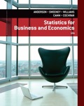
- b. Construct a bar chart for each question.
- c. Where are most adults living now?
- d. Where do most adults consider the ideal community?
- e. What changes in living areas would you expect to see if people moved from where they currently live to their ideal community?
a.
Construct the percent frequency distribution for each question.
Answer to Problem 9E
The percent frequency distribution for live now:
| Live now | Percent frequency |
| City | 32% |
| Suburb | 26% |
| Small Town | 26% |
| Rural Area | 16% |
| Total | 100 |
The percent frequency distribution for Ideal Community:
| Ideal Community | Percent frequency |
| City | 24% |
| Suburb | 25% |
| Small Town | 30% |
| Rural Area | 21% |
| Total | 100 |
Explanation of Solution
The given information is that Pew Research Centers Social & Demographic Trends project show that 46% of U.S adults would rather live in a different type of community than where they are living now. In the national survey of 2,260 adults are asked two types of questions. A sample of 100 respondents is provided. The respective living areas are City, Suburb, Small Town and Rural Area.
Calculation:
For live now:
Frequency:
The frequencies are calculated by using the tally mark.
Here, the number of times each class repeats is the frequency of that particular class.
Here, “City” is repeated for 32 times in the data set and thus 32 is the frequency for the category City.
Similarly, the frequency of remaining types of living area is given below:
| Live Now | Tally | Frequency |
| City | 32 | |
| Suburb | 26 | |
| Small Town | 26 | |
| Rural Area | 16 | |
| Total | 100 |
Relative frequency:
The general formula for the relative frequency is,
Therefore,
Similarly, the relative frequencies for the remaining types of living area are obtained below:
| Live Now | Frequency | Relative frequency |
| City | 32 | 0.32 |
| Suburb | 26 | 0.26 |
| Small Town | 26 | 0.26 |
| Rural Area | 16 | 0.16 |
| Total | 100 | 1.00 |
Percentage frequency distribution:
The general formula for the percent frequency is,
Therefore,
The percent frequencies for the remaining types of categories of living area for live now are obtained below:
| Live Now | Relative frequency | Percent frequency |
| City | 0.32 | 32% |
| Suburb | 0.26 | 26% |
| Small Town | 0.26 | 26% |
| Rural Area | 0.16 | 16% |
| Total | 1.00 | 100 |
For ideal community:
Here, city is repeated for 24 times in the data set and thus 24 is the frequency for the living area city.
Similarly, the frequency of remaining types of living area is given below:
| Ideal community | Tally | Frequency |
| City | 24 | |
| Suburb | 25 | |
| Small Town | 30 | |
| Rural Area | 21 | |
| Total | 100 |
Relative frequency:
Similarly, the relative frequencies for the remaining types of living area are obtained below:
| Ideal community | Frequency | Relative frequency |
| City | 24 | 0.24 |
| Suburb | 25 | 0.25 |
| Small Town | 30 | 0.30 |
| Rural Area | 21 | 0.21 |
| Total | 100 | 1.00 |
Percentage frequency distribution:
The percent frequencies for the remaining types of categories of living area of ideal community are obtained below:
| Ideal community | Relative Frequency | Percent frequency |
| City | 0.24 | 24% |
| Suburb | 0.25 | 25% |
| Small Town | 0.30 | 30% |
| Rural Area | 0.21 | 21% |
| Total | 1.00 | 100 |
b.
Construct the bar chart for each question.
Explanation of Solution
Output obtained from MINITAB software for live now is:
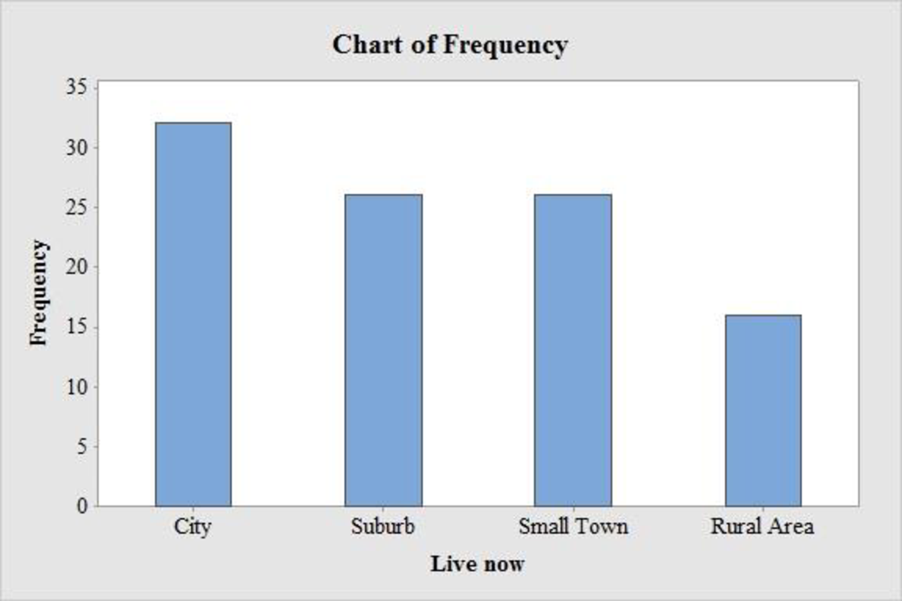
Output obtained from MINITAB software for Ideal community is:
Calculation:
For live now:
Software procedure:
Step by step procedure to draw the bar chart for bachelor’s degree using MINITAB software.
- Choose Graph > Bar Chart.
- From Bars represent, choose unique values from table.
- Choose Simple. Click OK.
- In Graph variables, enter the column of Live now.
- Click OK
- For ideal community:
Step by step procedure to draw the bar chart for Master’s degree using MINITAB software.
- Choose Graph > Bar Chart.
- From Bars represent, choose unique values from table.
- Choose Simple. Click OK.
- In Graph variables, enter the column of Ideal Community.
- Click OK
c.
Find the living area where the most adults are living now.
Answer to Problem 9E
The most adults in living now consider a City.
Explanation of Solution
For living now, the percentage for city is 32%, which is high when compared to other categories.
d.
Find the living area which the most adults are considered as an ideal community.
Answer to Problem 9E
The most adults consider the ideal community is a small town.
Explanation of Solution
For ideal, the percentage for small town is 30%, which is high when compared to other categories.
e.
Identify the changes in living areas would expect to see if people moved from where they currently live to their ideal community.
Explanation of Solution
The percentage changes can be obtained as follows:
Therefore,
The differences between two living areas are tabulated below:
| Living Area | Living now | Ideal community | Difference |
| City | 32% | 24% | –8% |
| Suburb | 26% | 25% | –1% |
| Small Town | 26% | 30% | 4% |
| Rural Area | 16% | 21% | 5% |
From the table, it is observed that the living areas “small town and rural area” has increased in percentage from “living now” to “ideal community” and the living areas “city and suburb” has decrease in percentage from “living now” to “ideal community”.
Want to see more full solutions like this?
Chapter 2 Solutions
EBK STATISTICS FOR BUSINESS & ECONOMICS


- Question 1 The data shown in Table 1 are and R values for 24 samples of size n = 5 taken from a process producing bearings. The measurements are made on the inside diameter of the bearing, with only the last three decimals recorded (i.e., 34.5 should be 0.50345). Table 1: Bearing Diameter Data Sample Number I R Sample Number I R 1 34.5 3 13 35.4 8 2 34.2 4 14 34.0 6 3 31.6 4 15 37.1 5 4 31.5 4 16 34.9 7 5 35.0 5 17 33.5 4 6 34.1 6 18 31.7 3 7 32.6 4 19 34.0 8 8 33.8 3 20 35.1 9 34.8 7 21 33.7 2 10 33.6 8 22 32.8 1 11 31.9 3 23 33.5 3 12 38.6 9 24 34.2 2 (a) Set up and R charts on this process. Does the process seem to be in statistical control? If necessary, revise the trial control limits. [15 pts] (b) If specifications on this diameter are 0.5030±0.0010, find the percentage of nonconforming bearings pro- duced by this process. Assume that diameter is normally distributed. [10 pts] 1arrow_forward4. (5 pts) Conduct a chi-square contingency test (test of independence) to assess whether there is an association between the behavior of the elderly person (did not stop to talk, did stop to talk) and their likelihood of falling. Below, please state your null and alternative hypotheses, calculate your expected values and write them in the table, compute the test statistic, test the null by comparing your test statistic to the critical value in Table A (p. 713-714) of your textbook and/or estimating the P-value, and provide your conclusions in written form. Make sure to show your work. Did not stop walking to talk Stopped walking to talk Suffered a fall 12 11 Totals 23 Did not suffer a fall | 2 Totals 35 37 14 46 60 Tarrow_forwardQuestion 2 Parts manufactured by an injection molding process are subjected to a compressive strength test. Twenty samples of five parts each are collected, and the compressive strengths (in psi) are shown in Table 2. Table 2: Strength Data for Question 2 Sample Number x1 x2 23 x4 x5 R 1 83.0 2 88.6 78.3 78.8 3 85.7 75.8 84.3 81.2 78.7 75.7 77.0 71.0 84.2 81.0 79.1 7.3 80.2 17.6 75.2 80.4 10.4 4 80.8 74.4 82.5 74.1 75.7 77.5 8.4 5 83.4 78.4 82.6 78.2 78.9 80.3 5.2 File Preview 6 75.3 79.9 87.3 89.7 81.8 82.8 14.5 7 74.5 78.0 80.8 73.4 79.7 77.3 7.4 8 79.2 84.4 81.5 86.0 74.5 81.1 11.4 9 80.5 86.2 76.2 64.1 80.2 81.4 9.9 10 75.7 75.2 71.1 82.1 74.3 75.7 10.9 11 80.0 81.5 78.4 73.8 78.1 78.4 7.7 12 80.6 81.8 79.3 73.8 81.7 79.4 8.0 13 82.7 81.3 79.1 82.0 79.5 80.9 3.6 14 79.2 74.9 78.6 77.7 75.3 77.1 4.3 15 85.5 82.1 82.8 73.4 71.7 79.1 13.8 16 78.8 79.6 80.2 79.1 80.8 79.7 2.0 17 82.1 78.2 18 84.5 76.9 75.5 83.5 81.2 19 79.0 77.8 20 84.5 73.1 78.2 82.1 79.2 81.1 7.6 81.2 84.4 81.6 80.8…arrow_forward
- Name: Lab Time: Quiz 7 & 8 (Take Home) - due Wednesday, Feb. 26 Contingency Analysis (Ch. 9) In lab 5, part 3, you will create a mosaic plot and conducted a chi-square contingency test to evaluate whether elderly patients who did not stop walking to talk (vs. those who did stop) were more likely to suffer a fall in the next six months. I have tabulated the data below. Answer the questions below. Please show your calculations on this or a separate sheet. Did not stop walking to talk Stopped walking to talk Totals Suffered a fall Did not suffer a fall Totals 12 11 23 2 35 37 14 14 46 60 Quiz 7: 1. (2 pts) Compute the odds of falling for each group. Compute the odds ratio for those who did not stop walking vs. those who did stop walking. Interpret your result verbally.arrow_forwardSolve please and thank you!arrow_forward7. In a 2011 article, M. Radelet and G. Pierce reported a logistic prediction equation for the death penalty verdicts in North Carolina. Let Y denote whether a subject convicted of murder received the death penalty (1=yes), for the defendant's race h (h1, black; h = 2, white), victim's race i (i = 1, black; i = 2, white), and number of additional factors j (j = 0, 1, 2). For the model logit[P(Y = 1)] = a + ß₁₂ + By + B²², they reported = -5.26, D â BD = 0, BD = 0.17, BY = 0, BY = 0.91, B = 0, B = 2.02, B = 3.98. (a) Estimate the probability of receiving the death penalty for the group most likely to receive it. [4 pts] (b) If, instead, parameters used constraints 3D = BY = 35 = 0, report the esti- mates. [3 pts] h (c) If, instead, parameters used constraints Σ₁ = Σ₁ BY = Σ; B = 0, report the estimates. [3 pts] Hint the probabilities, odds and odds ratios do not change with constraints.arrow_forward
- Solve please and thank you!arrow_forwardSolve please and thank you!arrow_forwardQuestion 1:We want to evaluate the impact on the monetary economy for a company of two types of strategy (competitive strategy, cooperative strategy) adopted by buyers.Competitive strategy: strategy characterized by firm behavior aimed at obtaining concessions from the buyer.Cooperative strategy: a strategy based on a problem-solving negotiating attitude, with a high level of trust and cooperation.A random sample of 17 buyers took part in a negotiation experiment in which 9 buyers adopted the competitive strategy, and the other 8 the cooperative strategy. The savings obtained for each group of buyers are presented in the pdf that i sent: For this problem, we assume that the samples are random and come from two normal populations of unknown but equal variances.According to the theory, the average saving of buyers adopting a competitive strategy will be lower than that of buyers adopting a cooperative strategy.a) Specify the population identifications and the hypotheses H0 and H1…arrow_forward
- You assume that the annual incomes for certain workers are normal with a mean of $28,500 and a standard deviation of $2,400. What’s the chance that a randomly selected employee makes more than $30,000?What’s the chance that 36 randomly selected employees make more than $30,000, on average?arrow_forwardWhat’s the chance that a fair coin comes up heads more than 60 times when you toss it 100 times?arrow_forwardSuppose that you have a normal population of quiz scores with mean 40 and standard deviation 10. Select a random sample of 40. What’s the chance that the mean of the quiz scores won’t exceed 45?Select one individual from the population. What’s the chance that his/her quiz score won’t exceed 45?arrow_forward
 Holt Mcdougal Larson Pre-algebra: Student Edition...AlgebraISBN:9780547587776Author:HOLT MCDOUGALPublisher:HOLT MCDOUGAL
 Big Ideas Math A Bridge To Success Algebra 1: Stu...AlgebraISBN:9781680331141Author:HOUGHTON MIFFLIN HARCOURTPublisher:Houghton Mifflin Harcourt
 Glencoe Algebra 1, Student Edition, 9780079039897...AlgebraISBN:9780079039897Author:CarterPublisher:McGraw Hill
 College Algebra (MindTap Course List)AlgebraISBN:9781305652231Author:R. David Gustafson, Jeff HughesPublisher:Cengage Learning