
Videos
Best description of the histogram’s shape.
Answer to Problem 38E
Best description of histogram’s shape would be skewed right.
Explanation of Solution
Given:
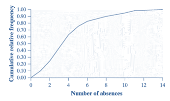
According to cumulative relative frequency graph,
Note that
The curve is very much steeper 0 and 4 as compared to that between 6 and 14.
Then
The distribution of the histogram should be skewed to the right, as most of the values of the data lie between 0 and 4 (where highest bar of the histogram appears) and very less values of the data lie between 6 and 14 that results in low bars tail to the right side of the highest bars.
Conclusion:
We can conclude that the best description of the histogram’s shape would be skewed right, because there are more data values between 0 and 4 as compared to that between 6 and 14. Therefore, the correct answer will be option (d).
Chapter 2 Solutions
PRACTICE OF STATISTICS F/AP EXAM
Additional Math Textbook Solutions
Basic Business Statistics, Student Value Edition
Calculus: Early Transcendentals (2nd Edition)
Elementary Statistics (13th Edition)
University Calculus: Early Transcendentals (4th Edition)
Thinking Mathematically (6th Edition)
Intro Stats, Books a la Carte Edition (5th Edition)


- Find the critical value for a left-tailed test using the F distribution with a 0.025, degrees of freedom in the numerator=12, and degrees of freedom in the denominator = 50. A portion of the table of critical values of the F-distribution is provided. Click the icon to view the partial table of critical values of the F-distribution. What is the critical value? (Round to two decimal places as needed.)arrow_forwardA retail store manager claims that the average daily sales of the store are $1,500. You aim to test whether the actual average daily sales differ significantly from this claimed value. You can provide your answer by inserting a text box and the answer must include: Null hypothesis, Alternative hypothesis, Show answer (output table/summary table), and Conclusion based on the P value. Showing the calculation is a must. If calculation is missing,so please provide a step by step on the answers Numerical answers in the yellow cellsarrow_forwardShow all workarrow_forward
- Show all workarrow_forwardplease find the answers for the yellows boxes using the information and the picture belowarrow_forwardA marketing agency wants to determine whether different advertising platforms generate significantly different levels of customer engagement. The agency measures the average number of daily clicks on ads for three platforms: Social Media, Search Engines, and Email Campaigns. The agency collects data on daily clicks for each platform over a 10-day period and wants to test whether there is a statistically significant difference in the mean number of daily clicks among these platforms. Conduct ANOVA test. You can provide your answer by inserting a text box and the answer must include: also please provide a step by on getting the answers in excel Null hypothesis, Alternative hypothesis, Show answer (output table/summary table), and Conclusion based on the P value.arrow_forward
 MATLAB: An Introduction with ApplicationsStatisticsISBN:9781119256830Author:Amos GilatPublisher:John Wiley & Sons Inc
 Probability and Statistics for Engineering and th...StatisticsISBN:9781305251809Author:Jay L. DevorePublisher:Cengage Learning
 Statistics for The Behavioral Sciences (MindTap C...StatisticsISBN:9781305504912Author:Frederick J Gravetter, Larry B. WallnauPublisher:Cengage Learning
 Elementary Statistics: Picturing the World (7th E...StatisticsISBN:9780134683416Author:Ron Larson, Betsy FarberPublisher:PEARSON
 The Basic Practice of StatisticsStatisticsISBN:9781319042578Author:David S. Moore, William I. Notz, Michael A. FlignerPublisher:W. H. Freeman
 Introduction to the Practice of StatisticsStatisticsISBN:9781319013387Author:David S. Moore, George P. McCabe, Bruce A. CraigPublisher:W. H. Freeman