
Videos
a.
Calculate the class width for the data on depths below surface grade at which significant artifacts were discovered.
a.
Answer to Problem 18P
The class width is calculated as 28.
Explanation of Solution
Calculation:
From the given data set, the largest data point is 200 and the smallest data point is 10.
Class Width:
The class width is calculated as follows:
b.
Create a table for frequency distribution with class limits, class boundaries, midpoints, frequencies, relative frequencies, and cumulative frequencies.
b.
Answer to Problem 18P
The class limits for a frequency table with 7 classes using class width 28 are 10-37, 38-65, 66-93, 94-121, 122-149, 150-177, and 178-205.
Explanation of Solution
Class limits:
Class limits are the maximum and minimum values in the class interval
Class Boundaries:
A class boundary is the midpoint between the upper limit of one class and the lower limit of the next class where the upper limit of the preceding class interval and the lower limit of the next class interval will be equal. The upper class boundary is calculated by adding 0.5 to the upper class limit and the lower class boundary is calculated by subtracting 0.5 from the lower class limit.
Midpoint:
The midpoint is calculated as given below:
Frequency:
Frequency is the number of data points that fall under each class.
Cumulative frequency:
Cumulative frequency is calculated by adding each frequency to the sum of preceding frequencies.
Relative Frequency:
Relative frequency is the ratio of frequency by the total number of data values.
The class width is 28. Hence, the lower class limit for the second class 261 is calculated by adding 25 to 236. Following this pattern, all the lower class limits are established. Then, the upper class limits are calculated.
The frequency distribution table is given below:
| Class Limits | Class Boundaries | Midpoints | Frequency | Relative Frequency | Cumulative Frequency |
| 10-37 | 9.5-37.5 |
23.5 | 7 | 7 | |
| 38-65 | 37.5-65.5 | 51.5 | 25 | 32 (=25+7) | |
| 66-93 | 65.5-93.5 | 79.5 | 26 | 58 (=26+32) | |
| 94-121 | 93.5-121.5 | 107.5 | 9 | 67 (=9+58) | |
| 122-149 | 121.5-149.5 | 135.5 | 5 | 72 (=5+67) | |
| 150-177 | 149.5-177.5 | 163.5 | 0 | 72 (=0+72) | |
| 178-205 | 177.5-205.5 | 191.5 | 1 | 73 (=1+72) |
c.
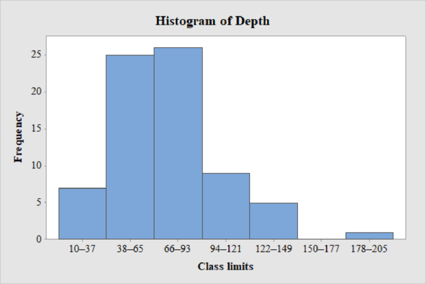
Create a histogram for the given data on depths below surface grade at which significant artifacts were discovered.
c.
Answer to Problem 18P
The frequency histogram for the data on depths below surface grade at which significant artifacts were discovered is shown below:
Explanation of Solution
Step-by-step procedure to draw the histogram using MINITAB software:
- Choose Graph > Bar Chart.
- From Bars represent, choose Values from a table.
- Under One column of values, choose Simple. Click OK.
- In Graph variables, enter the column of Frequency.
- In Categorical variable, enter the column of Class Limits.
- Click OK.
Thus, the histogram for depth is obtained.
d.
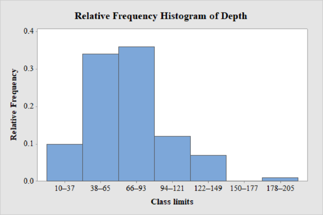
Construct a relative frequency histogram for the data on depths below surface grade at which significant artifacts were discovered.
d.
Answer to Problem 18P
The relative frequency histogram for the data on depths below surface grade at which significant artifacts were discovered is shown below:
Explanation of Solution
Step-by-step procedure to draw the histogram using MINITAB software:
- Choose Graph > Bar Chart.
- From Bars represent, choose Values from a table.
- Under One column of values, choose Simple. Click OK.
- In Graph variables, enter the column of Relative Frequency Class Limits.
- In Categorical variable, enter the column of Class Limits.
- Click OK.
Thus, the relative frequency histogram for depth is obtained.
e.
Identify the shape of distribution: uniform, mound shaped, symmetric, bimodal, skewed left, or skewed right.
e.
Explanation of Solution
From the histogram, the distribution of depths below surface grade at which significant artifacts were discovered is right-skewed and there is an unusual observation in the data.
f.
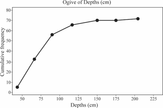
Create an ogive curve for the given data on depths below surface grade at which significant artifacts were discovered.
f.
Answer to Problem 18P
An ogive curve for the depths below surface grade at which significant artifacts were discovered is shown below:
Explanation of Solution
Step-by-step procedure to draw the Ogive curve:
- Draw X axis with data values ranging from 50 to 225.
- Label the X axis as Depths (cm).
- Draw Y axis with data values Cumulative frequency ranging from.0 to 80.
- Label the Y axis as Cumulative frequency.
- Plot the cumulative frequencies
- Join the points and draw an ogive curve.
Thus, an ogive curve for depth is obtained.
g.
Identify the characteristics about the depths below surface grade at which significant artifacts were discovered using the graphs.
g.
Explanation of Solution
The data values of depths below surface grade fall within 10 and 200.
The
The central value of the data is approximately 65.5.
From the histogram, it can be observed that the data is right-skewed and the outlier is 200.
Want to see more full solutions like this?
Chapter 2 Solutions
Understandable Statistics: Concepts and Methods


- ons 12. A sociologist hypothesizes that the crime rate is higher in areas with higher poverty rate and lower median income. She col- lects data on the crime rate (crimes per 100,000 residents), the poverty rate (in %), and the median income (in $1,000s) from 41 New England cities. A portion of the regression results is shown in the following table. Standard Coefficients error t stat p-value Intercept -301.62 549.71 -0.55 0.5864 Poverty 53.16 14.22 3.74 0.0006 Income 4.95 8.26 0.60 0.5526 a. b. Are the signs as expected on the slope coefficients? Predict the crime rate in an area with a poverty rate of 20% and a median income of $50,000. 3. Using data from 50 workarrow_forward2. The owner of several used-car dealerships believes that the selling price of a used car can best be predicted using the car's age. He uses data on the recent selling price (in $) and age of 20 used sedans to estimate Price = Po + B₁Age + ε. A portion of the regression results is shown in the accompanying table. Standard Coefficients Intercept 21187.94 Error 733.42 t Stat p-value 28.89 1.56E-16 Age -1208.25 128.95 -9.37 2.41E-08 a. What is the estimate for B₁? Interpret this value. b. What is the sample regression equation? C. Predict the selling price of a 5-year-old sedan.arrow_forwardian income of $50,000. erty rate of 13. Using data from 50 workers, a researcher estimates Wage = Bo+B,Education + B₂Experience + B3Age+e, where Wage is the hourly wage rate and Education, Experience, and Age are the years of higher education, the years of experience, and the age of the worker, respectively. A portion of the regression results is shown in the following table. ni ogolloo bash 1 Standard Coefficients error t stat p-value Intercept 7.87 4.09 1.93 0.0603 Education 1.44 0.34 4.24 0.0001 Experience 0.45 0.14 3.16 0.0028 Age -0.01 0.08 -0.14 0.8920 a. Interpret the estimated coefficients for Education and Experience. b. Predict the hourly wage rate for a 30-year-old worker with four years of higher education and three years of experience.arrow_forward
- 1. If a firm spends more on advertising, is it likely to increase sales? Data on annual sales (in $100,000s) and advertising expenditures (in $10,000s) were collected for 20 firms in order to estimate the model Sales = Po + B₁Advertising + ε. A portion of the regression results is shown in the accompanying table. Intercept Advertising Standard Coefficients Error t Stat p-value -7.42 1.46 -5.09 7.66E-05 0.42 0.05 8.70 7.26E-08 a. Interpret the estimated slope coefficient. b. What is the sample regression equation? C. Predict the sales for a firm that spends $500,000 annually on advertising.arrow_forwardCan you help me solve problem 38 with steps im stuck.arrow_forwardHow do the samples hold up to the efficiency test? What percentages of the samples pass or fail the test? What would be the likelihood of having the following specific number of efficiency test failures in the next 300 processors tested? 1 failures, 5 failures, 10 failures and 20 failures.arrow_forward
- The battery temperatures are a major concern for us. Can you analyze and describe the sample data? What are the average and median temperatures? How much variability is there in the temperatures? Is there anything that stands out? Our engineers’ assumption is that the temperature data is normally distributed. If that is the case, what would be the likelihood that the Safety Zone temperature will exceed 5.15 degrees? What is the probability that the Safety Zone temperature will be less than 4.65 degrees? What is the actual percentage of samples that exceed 5.25 degrees or are less than 4.75 degrees? Is the manufacturing process producing units with stable Safety Zone temperatures? Can you check if there are any apparent changes in the temperature pattern? Are there any outliers? A closer look at the Z-scores should help you in this regard.arrow_forwardNeed help pleasearrow_forwardPlease conduct a step by step of these statistical tests on separate sheets of Microsoft Excel. If the calculations in Microsoft Excel are incorrect, the null and alternative hypotheses, as well as the conclusions drawn from them, will be meaningless and will not receive any points. 4. One-Way ANOVA: Analyze the customer satisfaction scores across four different product categories to determine if there is a significant difference in means. (Hints: The null can be about maintaining status-quo or no difference among groups) H0 = H1=arrow_forward
- Please conduct a step by step of these statistical tests on separate sheets of Microsoft Excel. If the calculations in Microsoft Excel are incorrect, the null and alternative hypotheses, as well as the conclusions drawn from them, will be meaningless and will not receive any points 2. Two-Sample T-Test: Compare the average sales revenue of two different regions to determine if there is a significant difference. (Hints: The null can be about maintaining status-quo or no difference among groups; if alternative hypothesis is non-directional use the two-tailed p-value from excel file to make a decision about rejecting or not rejecting null) H0 = H1=arrow_forwardPlease conduct a step by step of these statistical tests on separate sheets of Microsoft Excel. If the calculations in Microsoft Excel are incorrect, the null and alternative hypotheses, as well as the conclusions drawn from them, will be meaningless and will not receive any points 3. Paired T-Test: A company implemented a training program to improve employee performance. To evaluate the effectiveness of the program, the company recorded the test scores of 25 employees before and after the training. Determine if the training program is effective in terms of scores of participants before and after the training. (Hints: The null can be about maintaining status-quo or no difference among groups; if alternative hypothesis is non-directional, use the two-tailed p-value from excel file to make a decision about rejecting or not rejecting the null) H0 = H1= Conclusion:arrow_forwardPlease conduct a step by step of these statistical tests on separate sheets of Microsoft Excel. If the calculations in Microsoft Excel are incorrect, the null and alternative hypotheses, as well as the conclusions drawn from them, will be meaningless and will not receive any points. The data for the following questions is provided in Microsoft Excel file on 4 separate sheets. Please conduct these statistical tests on separate sheets of Microsoft Excel. If the calculations in Microsoft Excel are incorrect, the null and alternative hypotheses, as well as the conclusions drawn from them, will be meaningless and will not receive any points. 1. One Sample T-Test: Determine whether the average satisfaction rating of customers for a product is significantly different from a hypothetical mean of 75. (Hints: The null can be about maintaining status-quo or no difference; If your alternative hypothesis is non-directional (e.g., μ≠75), you should use the two-tailed p-value from excel file to…arrow_forward
 Holt Mcdougal Larson Pre-algebra: Student Edition...AlgebraISBN:9780547587776Author:HOLT MCDOUGALPublisher:HOLT MCDOUGAL
 Glencoe Algebra 1, Student Edition, 9780079039897...AlgebraISBN:9780079039897Author:CarterPublisher:McGraw Hill
 Big Ideas Math A Bridge To Success Algebra 1: Stu...AlgebraISBN:9781680331141Author:HOUGHTON MIFFLIN HARCOURTPublisher:Houghton Mifflin Harcourt
 Functions and Change: A Modeling Approach to Coll...AlgebraISBN:9781337111348Author:Bruce Crauder, Benny Evans, Alan NoellPublisher:Cengage Learning