
Country which has unequal distribution of income-Australia or the United States.
Explanation of Solution
Here, as given the below table shows that the distribution of market income in Australia.
Table: 1
| Households | Market income (%) |
| Lowest 20% | 1 |
| Second 20% | 3 |
| Third 20% | 15 |
| Fourth 20% | 26 |
| Highest 20% | 55 |
Here, two sectors of the economy are Household and Business. Household sector owns all factors of production like land, labor and capital. These factors are required for production, which is carried out by business sector. Business sector has to pay price for getting these factors. Landowner will get rent, labor will receive wages and interest is paid to the owner of capital. Sum of the earnings from factors is known as household's market income.
Thus, household's income is the amount that he receives in a given period from factors.
In a country, the distribution of income is the important point. It indicates what percentage of income is flowing to a specific percentage of the total household. Total population is divided into few equal sized groups in ascending order from low income to high income. If total household is divided into five equal groups, then it is known as quintiles.
Then, in quintiles, each group consists of 20 percent of the total households. Considering market income percent of each group, income distribution table of an economy is formed.
Considering the market distribution of income in Australia as given in table 1 in the problem following cumulative distribution of income can be shown-
Cumulative Market Income distribution table of Australia:
| Groups | Percentage of | Cumulative percentage of | ||
| Households | Income | Households | Income | |
| A | Lowest 20% | 1 | 20% | 1 |
| B | Second 20% | 3 | 40% | 4 |
| C | Third 20% | 15 | 60% | 19 |
| D | Fourth 20% | 26 | 80% | 45 |
| E | Highest 20% | 55 | 100% | 100 |
In the above table: 2, entire households have been divided into five equal groups A to E. Each group consists of 20 percent of total households. There market income figures are taken from table 1.
Cumulative is the summation of all figures of the group and earlier groups. For group A, cumulative percentages and table: 2 figures are same since no other groups are available before group A. Cumulative figures of group B is the summation of percentage of group B and its earlier group A. Then, cumulative percentage of households is
In this manner, cumulative percentage of group C households is
Lorenz curve is a diagram, which reflects unequal distribution pattern of market income in an economy. The diagram is drawn below:
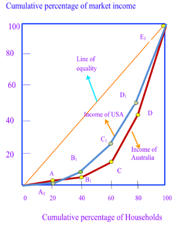
In the diagram, X-axis shows cumulative percentage of households and Y-axis measures the percentage of market income. Red curve is the actual percentage of income flowing to different subsections of people. Straight line is the curve when distribution is equal. Suppose 20% of total population receives exactly 20% of total income, then the distribution is equal. It will lie on a point of the linear curve. Hence, deviation of actual distribution line from equal distribution line will indicate level of unequal distribution. More the actual line deviates from linear line, more will be the level of unequal distribution.
Inequality of the distribution pattern of income in Australia and United states can be compared by drawing Lorenz curve of the two countries. In order to draw Lorenz curve of United States following data of the table are considered. The data below is the market income distribution of United States.
Cumulative Market income distribution table of United States:
| Groups | Percentage of | Cumulative percentage of | ||
| Households | Income | Households | Income | |
| A1 | Lowest 20% | 0.9 | 20% | 0.9 |
| B1 | Second 20% | 7.1 | 40% | 8.0 |
| C1 | Third 20% | 14.3 | 60% | 22.3 |
| D1 | Fourth 20% | 24.4 | 80% | 46.7 |
| E1 | Highest 20% | 53.3 | 100% | 100 |
Above data has been used to draw Lorenz curve of United States in the diagram above by a blue curve.
In the diagram, blue curve is closer to the straight line than red curve. Then, inequality in income distribution in United States is less than the inequality in income distribution at Australia.
Concept Introduction:
When there is huge difference between wealth of people living in a country, thereby leading to difference in living standard, is considered as inequality.
Want to see more full solutions like this?
Chapter 20 Solutions
EBK FOUNDATIONS OF ECONOMICS

- Sue is a sole proprietor of her own sewing business. Revenues are $150,000 per year and raw material (cloth, thread) costs are $130,000 per year. Sue pays herself a salary of $60,000 per year but gave up a job with a salary of $80,000 to run the business. ○ A. Her accounting profits are $0. Her economic profits are - $60,000. ○ B. Her accounting profits are $0. Her economic profits are - $40,000. ○ C. Her accounting profits are - $40,000. Her economic profits are - $60,000. ○ D. Her accounting profits are - $60,000. Her economic profits are -$40,000.arrow_forwardSelect a number that describes the type of firm organization indicated. Descriptions of Firm Organizations: 1. has one owner-manager who is personally responsible for all aspects of the business, including its debts 2. one type of partner takes part in managing the firm and is personally liable for the firm's actions and debts, and the other type of partner takes no part in the management of the firm and risks only the money that they have invested 3. owners are not personally responsible for anything that is done in the name of the firm 4. owned by the government but is usually under the direction of a more or less independent, state-appointed board 5. established with the explicit objective of providing goods or services but only in a manner that just covers its costs 6. has two or more joint owners, each of whom is personally responsible for all of the partnership's debts Type of Firm Organization a. limited partnership b. single proprietorship c. corporation Correct Numberarrow_forwardThe table below provides the total revenues and costs for a small landscaping company in a recent year. Total Revenues ($) 250,000 Total Costs ($) - wages and salaries 100,000 -risk-free return of 2% on owner's capital of $25,000 500 -interest on bank loan 1,000 - cost of supplies 27,000 - depreciation of capital equipment 8,000 - additional wages the owner could have earned in next best alternative 30,000 -risk premium of 4% on owner's capital of $25,000 1,000 The economic profits for this firm are ○ A. $83,000. B. $82,500. OC. $114,000. OD. $83,500. ○ E. $112,500.arrow_forward
- Output TFC ($) TVC ($) TC ($) (Q) 2 100 104 204 3 100 203 303 4 100 300 400 5 100 405 505 6 100 512 612 7 100 621 721 Given the information about short-run costs in the table above, we can conclude that the firm will minimize the average total cost of production when Q = (Round your response to the nearest whole number.)arrow_forwardThe following data show the total output for a firm when specified amounts of labour are combined with a fixed amount of capital. Assume that the wage per unit of labour is $20 and the cost of the capital is $100. Labour per unit of time 0 1 Total Output 0 25 T 2 3 4 5 75 137 212 267 The marginal product of labour is at its maximum when the firm changes the amount of labour hired from ○ A. 0 to 1 unit. ○ B. 3 to 4 units. OC. 2 to 3 units. OD. 1 to 2 units. ○ E. 4 to 5 units.arrow_forwardThe table below provides the annual revenues and costs for a family-owned firm producing catered meals. Total Revenues ($) 600,000 Total Costs ($) - wages and salaries 250,000 -risk-free return of 7% on owners' capital of $300,000 21,000 - rent 101,000 - depreciation of capital equipment 22,000 -risk premium of 9% on owners' capital of $300,000 27,000 - intermediate inputs 146,000 -forgone wages of owners in alternative employment -interest on bank loan 70,000 11,000 The implicit costs for this family-owned firm are ○ A. $70,000. OB. $97,000. OC. $589,000. OD. $118,000. ○ E. $48,000.arrow_forward
- Suppose a production function for a firm takes the following algebraic form: Q= 2KL - (0.3)L², where Q is the output of sweaters per day. Now suppose the firm is operating with 10 units of capital (K = 10) and 6 units of labour (L = 6). What is the output of sweaters? A. 64 sweaters per day OB. 49 sweaters per day OC. 109 sweaters per day OD. 72 sweaters per day OE. 118 sweaters per dayarrow_forward3. Consider a course allocation problem with strict and non-responsive preferences. Isthere a mechanism that is efficient and strategy-proof? If so, state the mechanismand show that it satisfies efficiency and strategyproofness. {hint serial dictatorship and show using example}4. Consider a course allocation problem with responsive preferences and at least 3students. Is there a mechanism that is efficient and strategy-proof that is not theSerial Dictatorship? If so, state the mechanism and show that it satisfies efficiencyand strategyproofness.5. Suggest a mechanism for allocating students to courses in a situation where preferences are non-responsive, and study its properties (efficiency and strategyproofness). Please be creativearrow_forward3. Consider a course allocation problem with strict and non-responsive preferences. Isthere a mechanism that is efficient and strategy-proof? If so, state the mechanismand show that it satisfies efficiency and strategyproofness. {hint serial dictatorship}4. Consider a course allocation problem with responsive preferences and at least 3students. Is there a mechanism that is efficient and strategy-proof that is not theSerial Dictatorship? If so, state the mechanism and show that it satisfies efficiencyand strategyproofness.5. Suggest a mechanism for allocating students to courses in a situation where preferences are non-responsive, and study its properties (efficiency and strategyproofness). Please be creativearrow_forward
 Economics (MindTap Course List)EconomicsISBN:9781337617383Author:Roger A. ArnoldPublisher:Cengage Learning
 Microeconomics: Private and Public Choice (MindTa...EconomicsISBN:9781305506893Author:James D. Gwartney, Richard L. Stroup, Russell S. Sobel, David A. MacphersonPublisher:Cengage Learning
 Economics: Private and Public Choice (MindTap Cou...EconomicsISBN:9781305506725Author:James D. Gwartney, Richard L. Stroup, Russell S. Sobel, David A. MacphersonPublisher:Cengage Learning
 Principles of Economics (MindTap Course List)EconomicsISBN:9781305585126Author:N. Gregory MankiwPublisher:Cengage Learning
 Principles of Microeconomics (MindTap Course List)EconomicsISBN:9781305971493Author:N. Gregory MankiwPublisher:Cengage Learning