Calculus
6th Edition
ISBN: 9781465208880
Author: SMITH KARL J, STRAUSS MONTY J, TODA MAGDALENA DANIELE
Publisher: Kendall Hunt Publishing
expand_more
expand_more
format_list_bulleted
Concept explainers
Videos
Question
Chapter 2, Problem 86SP
(a)
To determine
To graph : Below data points:
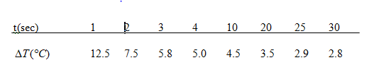
To calculate:Temperature difference
(b)
To determine
To graph : Below data points:
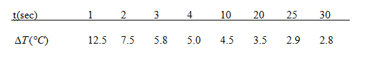
To calculate: Exposure time t, when temperature difference i.e
Expert Solution & Answer
Want to see the full answer?
Check out a sample textbook solution
Students have asked these similar questions
Please focus on problem ii.
Please focus on problem x.
Please focus on vii.
Chapter 2 Solutions
Calculus
Ch. 2.1 - Prob. 1PSCh. 2.1 - Prob. 2PSCh. 2.1 - Prob. 3PSCh. 2.1 - Prob. 4PSCh. 2.1 - Prob. 5PSCh. 2.1 - Prob. 6PSCh. 2.1 - Prob. 7PSCh. 2.1 - Prob. 8PSCh. 2.1 - Prob. 9PSCh. 2.1 - Prob. 10PS
Ch. 2.1 - Prob. 11PSCh. 2.1 - Prob. 12PSCh. 2.1 - Prob. 13PSCh. 2.1 - Prob. 14PSCh. 2.1 - Prob. 15PSCh. 2.1 - Prob. 16PSCh. 2.1 - Prob. 17PSCh. 2.1 - Prob. 18PSCh. 2.1 - Prob. 19PSCh. 2.1 - Prob. 20PSCh. 2.1 - Prob. 21PSCh. 2.1 - Prob. 22PSCh. 2.1 - Prob. 23PSCh. 2.1 - Prob. 24PSCh. 2.1 - Prob. 25PSCh. 2.1 - Prob. 26PSCh. 2.1 - Prob. 27PSCh. 2.1 - Prob. 28PSCh. 2.1 - Prob. 29PSCh. 2.1 - Prob. 30PSCh. 2.1 - Prob. 31PSCh. 2.1 - Prob. 32PSCh. 2.1 - Prob. 33PSCh. 2.1 - Prob. 34PSCh. 2.1 - Prob. 35PSCh. 2.1 - Prob. 36PSCh. 2.1 - Prob. 37PSCh. 2.1 - Prob. 38PSCh. 2.1 - Prob. 39PSCh. 2.1 - Prob. 40PSCh. 2.1 - Prob. 41PSCh. 2.1 - Prob. 42PSCh. 2.1 - Prob. 43PSCh. 2.1 - Prob. 44PSCh. 2.1 - Prob. 45PSCh. 2.1 - Prob. 46PSCh. 2.1 - Prob. 47PSCh. 2.1 - Prob. 48PSCh. 2.1 - Prob. 49PSCh. 2.1 - Prob. 50PSCh. 2.1 - Prob. 51PSCh. 2.1 - Prob. 52PSCh. 2.1 - Prob. 53PSCh. 2.1 - Prob. 54PSCh. 2.1 - Prob. 55PSCh. 2.1 - Prob. 56PSCh. 2.1 - Prob. 57PSCh. 2.1 - Prob. 58PSCh. 2.1 - Prob. 59PSCh. 2.1 - Prob. 60PSCh. 2.2 - Prob. 1PSCh. 2.2 - Prob. 2PSCh. 2.2 - Prob. 3PSCh. 2.2 - Prob. 4PSCh. 2.2 - Prob. 5PSCh. 2.2 - Prob. 6PSCh. 2.2 - Prob. 7PSCh. 2.2 - Prob. 8PSCh. 2.2 - Prob. 9PSCh. 2.2 - Prob. 10PSCh. 2.2 - Prob. 11PSCh. 2.2 - Prob. 12PSCh. 2.2 - Prob. 13PSCh. 2.2 - Prob. 14PSCh. 2.2 - Prob. 15PSCh. 2.2 - Prob. 16PSCh. 2.2 - Prob. 17PSCh. 2.2 - Prob. 18PSCh. 2.2 - Prob. 19PSCh. 2.2 - Prob. 20PSCh. 2.2 - Prob. 21PSCh. 2.2 - Prob. 22PSCh. 2.2 - Prob. 23PSCh. 2.2 - Prob. 24PSCh. 2.2 - Prob. 25PSCh. 2.2 - Prob. 26PSCh. 2.2 - Prob. 27PSCh. 2.2 - Prob. 28PSCh. 2.2 - Prob. 29PSCh. 2.2 - Prob. 30PSCh. 2.2 - Prob. 31PSCh. 2.2 - Prob. 32PSCh. 2.2 - Prob. 33PSCh. 2.2 - Prob. 34PSCh. 2.2 - Prob. 35PSCh. 2.2 - Prob. 36PSCh. 2.2 - Prob. 37PSCh. 2.2 - Prob. 38PSCh. 2.2 - Prob. 39PSCh. 2.2 - Prob. 40PSCh. 2.2 - Prob. 41PSCh. 2.2 - Prob. 42PSCh. 2.2 - Prob. 43PSCh. 2.2 - Prob. 44PSCh. 2.2 - Prob. 45PSCh. 2.2 - Prob. 46PSCh. 2.2 - Prob. 47PSCh. 2.2 - Prob. 48PSCh. 2.2 - Prob. 49PSCh. 2.2 - Prob. 50PSCh. 2.2 - Prob. 51PSCh. 2.2 - Prob. 52PSCh. 2.2 - Prob. 53PSCh. 2.2 - Prob. 54PSCh. 2.2 - Prob. 55PSCh. 2.2 - Prob. 56PSCh. 2.2 - Prob. 57PSCh. 2.2 - Prob. 58PSCh. 2.2 - Prob. 59PSCh. 2.2 - Prob. 60PSCh. 2.3 - Prob. 1PSCh. 2.3 - Prob. 2PSCh. 2.3 - Prob. 3PSCh. 2.3 - Prob. 4PSCh. 2.3 - Prob. 5PSCh. 2.3 - Prob. 6PSCh. 2.3 - Prob. 7PSCh. 2.3 - Prob. 8PSCh. 2.3 - Prob. 9PSCh. 2.3 - Prob. 10PSCh. 2.3 - Prob. 11PSCh. 2.3 - Prob. 12PSCh. 2.3 - Prob. 13PSCh. 2.3 - Prob. 14PSCh. 2.3 - Prob. 15PSCh. 2.3 - Prob. 16PSCh. 2.3 - Prob. 17PSCh. 2.3 - Prob. 18PSCh. 2.3 - Prob. 19PSCh. 2.3 - Prob. 20PSCh. 2.3 - Prob. 21PSCh. 2.3 - Prob. 22PSCh. 2.3 - Prob. 23PSCh. 2.3 - Prob. 24PSCh. 2.3 - Prob. 25PSCh. 2.3 - Prob. 26PSCh. 2.3 - Prob. 27PSCh. 2.3 - Prob. 28PSCh. 2.3 - Prob. 29PSCh. 2.3 - Prob. 30PSCh. 2.3 - Prob. 31PSCh. 2.3 - Prob. 32PSCh. 2.3 - Prob. 33PSCh. 2.3 - Prob. 34PSCh. 2.3 - Prob. 35PSCh. 2.3 - Prob. 36PSCh. 2.3 - Prob. 37PSCh. 2.3 - Prob. 38PSCh. 2.3 - Prob. 39PSCh. 2.3 - Prob. 40PSCh. 2.3 - Prob. 41PSCh. 2.3 - Prob. 42PSCh. 2.3 - Prob. 43PSCh. 2.3 - Prob. 44PSCh. 2.3 - Prob. 45PSCh. 2.3 - Prob. 46PSCh. 2.3 - Prob. 47PSCh. 2.3 - Prob. 48PSCh. 2.3 - Prob. 49PSCh. 2.3 - Prob. 50PSCh. 2.3 - Prob. 51PSCh. 2.3 - Prob. 52PSCh. 2.3 - Prob. 53PSCh. 2.3 - Prob. 54PSCh. 2.3 - Prob. 56PSCh. 2.3 - Prob. 57PSCh. 2.3 - Prob. 58PSCh. 2.3 - Prob. 59PSCh. 2.3 - Prob. 60PSCh. 2.4 - Prob. 1PSCh. 2.4 - Prob. 2PSCh. 2.4 - Prob. 3PSCh. 2.4 - Prob. 4PSCh. 2.4 - Prob. 5PSCh. 2.4 - Prob. 6PSCh. 2.4 - Prob. 7PSCh. 2.4 - Prob. 8PSCh. 2.4 - Prob. 9PSCh. 2.4 - Prob. 10PSCh. 2.4 - Prob. 11PSCh. 2.4 - Prob. 12PSCh. 2.4 - Prob. 13PSCh. 2.4 - Prob. 14PSCh. 2.4 - Prob. 15PSCh. 2.4 - Prob. 16PSCh. 2.4 - Prob. 17PSCh. 2.4 - Prob. 18PSCh. 2.4 - Prob. 19PSCh. 2.4 - Prob. 20PSCh. 2.4 - Prob. 21PSCh. 2.4 - Prob. 22PSCh. 2.4 - Prob. 23PSCh. 2.4 - Prob. 24PSCh. 2.4 - Prob. 25PSCh. 2.4 - Prob. 26PSCh. 2.4 - Prob. 27PSCh. 2.4 - Prob. 28PSCh. 2.4 - Prob. 29PSCh. 2.4 - Prob. 30PSCh. 2.4 - Prob. 31PSCh. 2.4 - Prob. 32PSCh. 2.4 - Prob. 33PSCh. 2.4 - Prob. 34PSCh. 2.4 - Prob. 35PSCh. 2.4 - Prob. 36PSCh. 2.4 - Prob. 37PSCh. 2.4 - Prob. 38PSCh. 2.4 - Prob. 39PSCh. 2.4 - Prob. 40PSCh. 2.4 - Prob. 41PSCh. 2.4 - Prob. 42PSCh. 2.4 - Prob. 43PSCh. 2.4 - Prob. 44PSCh. 2.4 - Prob. 45PSCh. 2.4 - Prob. 46PSCh. 2.4 - Prob. 47PSCh. 2.4 - Prob. 48PSCh. 2.4 - Prob. 49PSCh. 2.4 - Prob. 50PSCh. 2.4 - Prob. 51PSCh. 2.4 - Prob. 52PSCh. 2.4 - Prob. 53PSCh. 2.4 - Prob. 54PSCh. 2.4 - Prob. 55PSCh. 2.4 - Prob. 56PSCh. 2.4 - Prob. 57PSCh. 2.4 - Prob. 58PSCh. 2.4 - Prob. 59PSCh. 2.4 - Prob. 60PSCh. 2 - Prob. 1PECh. 2 - Prob. 2PECh. 2 - Prob. 3PECh. 2 - Prob. 4PECh. 2 - Prob. 5PECh. 2 - Prob. 6PECh. 2 - Prob. 7PECh. 2 - Prob. 8PECh. 2 - Prob. 9PECh. 2 - Prob. 10PECh. 2 - Prob. 11PECh. 2 - Prob. 12PECh. 2 - Prob. 13PECh. 2 - Prob. 14PECh. 2 - Prob. 15PECh. 2 - Prob. 16PECh. 2 - Prob. 17PECh. 2 - Prob. 18PECh. 2 - Prob. 19PECh. 2 - Prob. 20PECh. 2 - Prob. 21PECh. 2 - Prob. 22PECh. 2 - Prob. 23PECh. 2 - Prob. 24PECh. 2 - Prob. 25PECh. 2 - Prob. 26PECh. 2 - Prob. 27PECh. 2 - Prob. 28PECh. 2 - Prob. 29PECh. 2 - Prob. 30PECh. 2 - Prob. 1SPCh. 2 - Prob. 2SPCh. 2 - Prob. 3SPCh. 2 - Prob. 4SPCh. 2 - Prob. 5SPCh. 2 - Prob. 6SPCh. 2 - Prob. 7SPCh. 2 - Prob. 8SPCh. 2 - Prob. 9SPCh. 2 - Prob. 10SPCh. 2 - Prob. 11SPCh. 2 - Prob. 12SPCh. 2 - Prob. 13SPCh. 2 - Prob. 14SPCh. 2 - Prob. 15SPCh. 2 - Prob. 16SPCh. 2 - Prob. 17SPCh. 2 - Prob. 18SPCh. 2 - Prob. 19SPCh. 2 - Prob. 20SPCh. 2 - Prob. 21SPCh. 2 - Prob. 22SPCh. 2 - Prob. 23SPCh. 2 - Prob. 24SPCh. 2 - Prob. 25SPCh. 2 - Prob. 26SPCh. 2 - Prob. 27SPCh. 2 - Prob. 28SPCh. 2 - Prob. 29SPCh. 2 - Prob. 30SPCh. 2 - Prob. 31SPCh. 2 - Prob. 32SPCh. 2 - Prob. 33SPCh. 2 - Prob. 34SPCh. 2 - Prob. 35SPCh. 2 - Prob. 36SPCh. 2 - Prob. 37SPCh. 2 - Prob. 38SPCh. 2 - Prob. 39SPCh. 2 - Prob. 40SPCh. 2 - Prob. 41SPCh. 2 - Prob. 42SPCh. 2 - Prob. 43SPCh. 2 - Prob. 44SPCh. 2 - Prob. 45SPCh. 2 - Prob. 46SPCh. 2 - Prob. 47SPCh. 2 - Prob. 48SPCh. 2 - Prob. 49SPCh. 2 - Prob. 50SPCh. 2 - Prob. 51SPCh. 2 - Prob. 52SPCh. 2 - Prob. 53SPCh. 2 - Prob. 54SPCh. 2 - Prob. 55SPCh. 2 - Prob. 56SPCh. 2 - Prob. 57SPCh. 2 - Prob. 58SPCh. 2 - Prob. 59SPCh. 2 - Prob. 60SPCh. 2 - Prob. 61SPCh. 2 - Prob. 62SPCh. 2 - Prob. 63SPCh. 2 - Prob. 64SPCh. 2 - Prob. 65SPCh. 2 - Prob. 66SPCh. 2 - Prob. 67SPCh. 2 - Prob. 68SPCh. 2 - Prob. 69SPCh. 2 - Prob. 70SPCh. 2 - Prob. 71SPCh. 2 - Prob. 72SPCh. 2 - Prob. 73SPCh. 2 - Prob. 74SPCh. 2 - Prob. 75SPCh. 2 - Prob. 76SPCh. 2 - Prob. 77SPCh. 2 - Prob. 78SPCh. 2 - Prob. 79SPCh. 2 - Prob. 80SPCh. 2 - Prob. 81SPCh. 2 - Prob. 82SPCh. 2 - Prob. 83SPCh. 2 - Prob. 84SPCh. 2 - Prob. 85SPCh. 2 - Prob. 86SPCh. 2 - Prob. 87SPCh. 2 - Prob. 88SPCh. 2 - Prob. 89SPCh. 2 - Prob. 90SPCh. 2 - Prob. 91SPCh. 2 - Prob. 92SPCh. 2 - Prob. 93SPCh. 2 - Prob. 94SPCh. 2 - Prob. 95SPCh. 2 - Prob. 96SPCh. 2 - Prob. 97SPCh. 2 - Prob. 98SPCh. 2 - Prob. 99SP
Knowledge Booster


Learn more about
Need a deep-dive on the concept behind this application? Look no further. Learn more about this topic, calculus and related others by exploring similar questions and additional content below.Similar questions
- Please focus on ix.arrow_forwardPlease focus on vi.arrow_forward的 v If A is an n x n matrix that is not invertible, then A. rank(A) = n C. det(A) = 0 B. Reduced row-echelon form of A = In D. AB BA= In for some matrix B 63°F Partly sunny Q Search 3 $ 4 40 FS 96 S W E A S T FG S Y & コ B ㅁ F G H J 4 Z X C V B N M 9 H V FIB - FIB ㅁ P L ว DELETE BACHSPACE LOCK L ? PAUSE ALT CTRL ENTER 7 2:20 PM 4/14/2025 HOME J INSERT SHIFT END 5arrow_forward
- i Compute the given determinant by cofactor expansions. At each step, choose a row or columnthat involves the least amount of computation.7 6 8 40 0 0 68 7 9 30 4 0 5arrow_forwardi Compute the inverse of the matrix below using row operations. Please show your work.1 0 −2−3 1 42 −3 4 This is a 3*3 matrix. First row is 1 0 -2.arrow_forwardSolve the system of equations below by applying row operations on the corresponding aug-mented matrix to convert it to the reduced row-echelon form. Write the solutions using freevariables as parameters.x1 + 3x2 + x3 = 1−4x1 − 9x2 + 2x3 = −1−3x2 − 6x3 = −3arrow_forward
arrow_back_ios
SEE MORE QUESTIONS
arrow_forward_ios
Recommended textbooks for you
 Algebra & Trigonometry with Analytic GeometryAlgebraISBN:9781133382119Author:SwokowskiPublisher:Cengage
 Mathematics For Machine TechnologyAdvanced MathISBN:9781337798310Author:Peterson, John.Publisher:Cengage Learning,
 College Algebra (MindTap Course List)AlgebraISBN:9781305652231Author:R. David Gustafson, Jeff HughesPublisher:Cengage Learning
Algebra & Trigonometry with Analytic Geometry
Algebra
ISBN:9781133382119
Author:Swokowski
Publisher:Cengage
Mathematics For Machine Technology
Advanced Math
ISBN:9781337798310
Author:Peterson, John.
Publisher:Cengage Learning,
College Algebra (MindTap Course List)
Algebra
ISBN:9781305652231
Author:R. David Gustafson, Jeff Hughes
Publisher:Cengage Learning
Continuous Probability Distributions - Basic Introduction; Author: The Organic Chemistry Tutor;https://www.youtube.com/watch?v=QxqxdQ_g2uw;License: Standard YouTube License, CC-BY
Probability Density Function (p.d.f.) Finding k (Part 1) | ExamSolutions; Author: ExamSolutions;https://www.youtube.com/watch?v=RsuS2ehsTDM;License: Standard YouTube License, CC-BY
Find the value of k so that the Function is a Probability Density Function; Author: The Math Sorcerer;https://www.youtube.com/watch?v=QqoCZWrVnbA;License: Standard Youtube License