Refer to the Lincolnville School District bus data. Select the variable referring to the number of miles traveled since the last maintenance, and then organize these data into a frequency distribution.
- a. What is a typical amount of miles traveled? What is the
range ? - b. Comment on the shape of the distribution. Are there any outliers in terms of miles driven?
- c. Draw a cumulative relative frequency distribution. Forty percent of the buses were driven fewer than how many miles? How many buses were driven less than 10,500 miles?
- d. Refer to the variables regarding the bus manufacturer and the bus capacity. Draw a pie chart of each variable and write a description of your results.
a.
Obtain a frequency distribution for the variable Team salary.
Find the typical amount of miles travelled.
Find the range of the miles.
Answer to Problem 53DA
The frequency distribution for the salary is given below:
| Miles | Frequency |
Cumulative frequency |
| 9,900-10,200 | 8 | 8 |
| 10,200-10,500 | 8 | 16 |
| 10,500-10,800 | 11 | 27 |
| 10,800-11,100 | 8 | 35 |
| 11,100-11,400 | 13 | 48 |
| 11,400-11,700 | 12 | 60 |
| 11,700-12,000 | 20 | 80 |
| Total | 80 |
The typical mile driven is about 11,100 miles.
The range of the salaries is 2,100 miles.
Explanation of Solution
Selection of the number of classes:
The “2 to the k rule” suggests that the number of classes is the smallest value of k, where
It is given that the data set consists of 80 observations. The value of k can be obtained as follows:
Here,
Therefore, the number of classes for the given data set is 7.
From the data set, the maximum and minimum values are 11,973 and 10,000, respectively.
The formula for the class interval is given as follows:
Where, i is the class interval and k is the number of classes.
Therefore, the class interval for the given data can be obtained as follows:
In practice, the class interval size is usually rounded up to some convenient number. Therefore, the reasonable class interval is 300.
Frequency distribution:
The frequency table is a collection of mutually exclusive and exhaustive classes, which shows the number of observations in each class.
Since the minimum value is 10,000 and the class interval is 300, the first class would be 9,900-10,200. The frequency distribution for miles can be constructed as follows:
| Miles | Frequency |
Cumulative frequency |
| 9,900-10,200 | 8 | 8 |
| 10,200-10,500 | 8 | |
| 10,500-10,800 | 11 | |
| 10,800-11,100 | 8 | |
| 11,100-11,400 | 13 | |
| 11,400-11,700 | 12 | |
| 11,700-12,000 | 20 | |
| Total | 80 |
From the above frequency distribution, the typical miles driven is about 11,100 miles.
The range of miles is from 12,000 to 9,900 million dollars. Thus, the range of salaries is 2,100 miles.
b.
Make a comment on the shape of the distribution.
Check whether there are any outliers in terms of miles driven.
Answer to Problem 53DA
Thus, the distribution of miles is negatively skewed.
There are no outliers detected in the data.
Explanation of Solution
From the frequency distribution in Part (a), the large number of frequencies occurred in last three classes. Therefore, the distribution of miles is negatively skewed.
There are no observations much higher or much lower than the remaining observations. Thus, no outliers were detected in the data.
c.
Create a cumulative relative frequency polygon for the frequency distribution.
Identify the distance for which less than 40% of the buses are driven.
Find the number of buses that drives less than 10,500 miles.
Answer to Problem 53DA
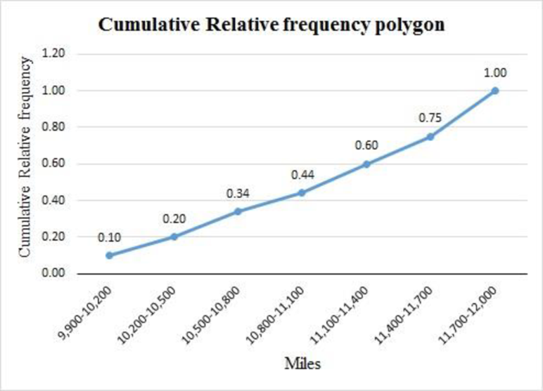
The cumulative frequency polygon for the given data is as follows:

There are 40% of the buses driven less than 1,100 miles.
There are 16 of the buses driven less than 10,500 miles.
Explanation of Solution
For the given data set, the cumulative relative frequency table with midpoints of classes is obtained as follows:
| Miles | Midpoint |
Cumulative frequency |
Relative cumulative frequency |
| 9,900-10,200 | 8 | ||
| 10,200-10,500 | 16 | ||
| 10,500-10,800 | 27 | ||
| 10,800-11,100 | 35 | ||
| 11,100-11,400 | 48 | ||
| 11,400-11,700 | 60 | ||
| 11,700-12,000 | 80 |
The cumulative relative frequency polygon for the given data can be drawn using EXCEL:
Step-by-step procedure to obtain the frequency polygon using EXCEL:
- Enter the column of midpoints along with the cumulative relative frequency column.
- Select the total data range with labels.
- Go to Insert > Charts > line chart.
- Select the appropriate line chart.
- Click OK.
From the above cumulative relative frequency polygon, 40% of the buses are driven less than 1,100 miles.
There are 16 of the buses driven less than 10,500 miles.
d.
Create pie charts for the variables Manufacturer and Capacity.
Answer to Problem 53DA
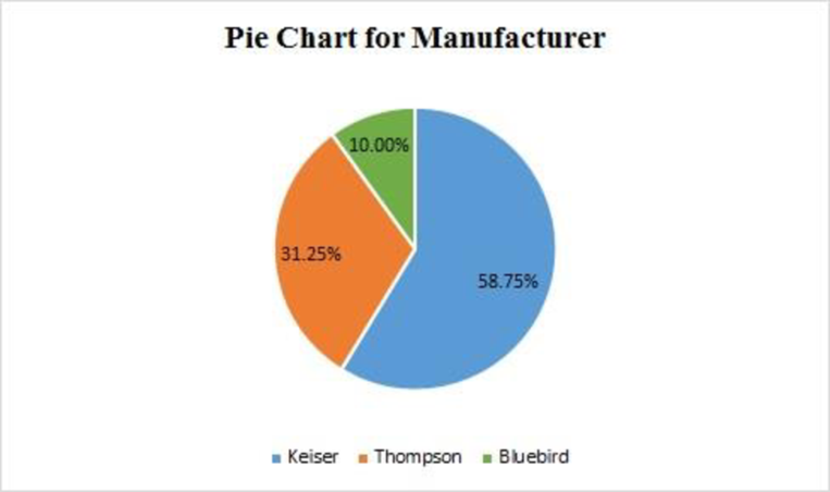
The pie chart for the variable Manufacturer is given as follows:

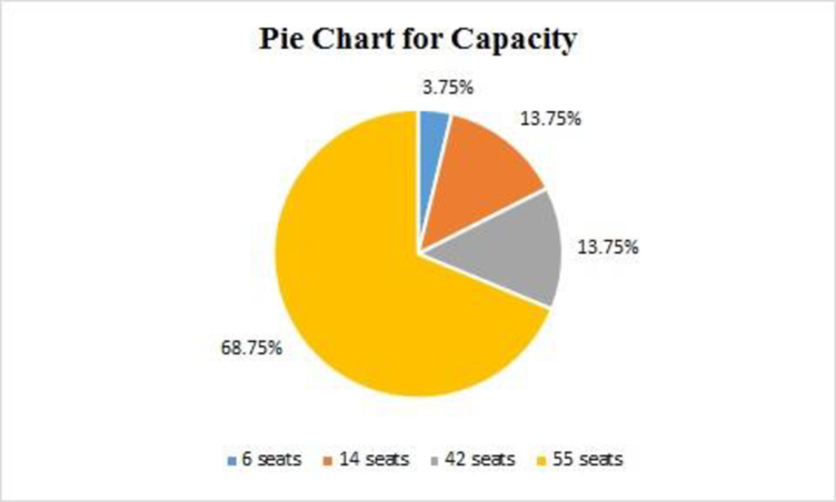
The pie chart for the variable Capacity is given as follows:

Explanation of Solution
Manufacturer:
From the data set, there are three manufacturers in the variable Manufacturer, their corresponding frequencies and percentages of the frequencies are given in the below table:
| Manufacturer | Frequency | % of frequency |
| Bluebird | 47 | |
| Keiser | 25 | |
| Thompson | 8 | |
| Total | 80 |
Step-by-step procedure to obtain the pie chart using EXCEL:
- Enter the Manufacturer column along with the corresponding percentage of frequencies.
- Select the total data range with labels.
- Go to Insert > Charts > Pie chart.
- Select the appropriate Pie chart.
- Click OK.
Capacity:
From the data set, there are four capacities of seats in the variable Capacity, their corresponding frequencies and percentages of the frequencies are given in the below table:
| Capacity | Frequency | % of frequency |
| 6 seats | 3 | |
| 14 seats | 11 | |
| 42 seats | 11 | |
| 55 seats | 55 | |
| Total | 80 |
Step-by-step procedure to obtain the pie chart using EXCEL:
- Enter the Capacity column along with the corresponding percentage of frequencies.
- Select the total data range with labels.
- Go to Insert > Charts > Pie chart.
- Select the appropriate Pie chart.
- Click OK.
Want to see more full solutions like this?
Chapter 2 Solutions
EBK STATISTICAL TECHNIQUES IN BUSINESS
- 1 (Expected Shortfall) Suppose the price of an asset Pt follows a normal random walk, i.e., Pt = Po+r₁ + ... + rt with r₁, r2,... being IID N(μ, o²). Po+r1+. ⚫ Suppose the VaR of rt is VaRq(rt) at level q, find the VaR of the price in T days, i.e., VaRq(Pt – Pt–T). - • If ESq(rt) = A, find ES₁(Pt – Pt–T).arrow_forward2 (Normal Distribution) Let rt be a log return. Suppose that r₁, 2, ... are IID N(0.06, 0.47). What is the distribution of rt (4) = rt + rt-1 + rt-2 + rt-3? What is P(rt (4) < 2)? What is the covariance between r2(2) = 1 + 12 and 13(2) = r² + 13? • What is the conditional distribution of r₁(3) = rt + rt-1 + rt-2 given rt-2 = 0.6?arrow_forward3 (Sharpe-ratio) Suppose that X1, X2,..., is a lognormal geometric random walk with parameters (μ, o²). Specifically, suppose that X = Xo exp(rı + ...Tk), where Xo is a fixed constant and r1, T2, ... are IID N(μ, o²). Find the Sharpe-ratios of rk and log(Xk) — log(Xo) respectively, assuming the risk free return is 0.arrow_forward
- i need help with question 2arrow_forward4 (Value-at-Risk and Expected Shortfall) Suppose X Find VaR0.02(X) and ES0.02 (X). ~ Uniform(-1, 1).arrow_forward亚 ח Variables Name avgdr employ educ exerany Label AVG ALCOHOLIC DRINKS PER DAY IN PAST 30 EMPLOYMENT STATUS EDUCATION LEVEL EXERCISE IN PAST 30 DAYSarrow_forward
- Variables Name wage hours IQ KWW educ exper tenure age married black south urban sibs brthord meduc feduc Label monthly earnings average weekly hours IQ score knowledge of world work score years of education years of work experience years with current employer age in years =1 if married =1 if black =1 if live in south =1 if live in SMSA number of siblings birth order mother's education father's educationarrow_forwardInformation for questions 4 • • Please Download "wages" from Canvas (the link to this dataset is right below the HWA1 questions - it is a Microsoft excel worksheet) and store it in your favorite folder. It contains 797 observations and 16 variables. The "state" variable gives the names of the states involved in this dataset. • You need to have excel on your computer to open this dataset. i. You should use File > Import > Excel Spreadsheet etc. as done in class 3 convert this file into a Stata dataset. Once you are done, write the final STATA code that makes the transformation of an excel file to a STATA file possible. ii. Write a code that will close the log file that has been open since Question 1 part ii.arrow_forwardThe mean, variance, skewness and kurtosis of a dataset are given as - Mean = 15, Variance = 20, SKewness = 1.5 and Kurtosis = 3.5 calculate the first four raw moments. (Note- Please include as much detailed solution/steps in the solution to understand, Thank you!)arrow_forward
- Write codes to perform the functions in each of these cases i. ii. Apply cd command to tell STATA the filepath associated with your "favorite folder" (use the same name for the favorite folder that we have been using in class) Apply log using command to tell stata that you are creating a log file to record the codes and the outcomes of these codes. Make sure your log file is called loghwa1_W25.smcl. Do not forget to include the replace option. iii. Get help for the "regress" command & include a screenshot of the outcome of this code iv. V. Open a stata file stored in STATA memory called pop2000.dta Continue from question iv. Save this file in your favorite folder (current working directory) using a different name & a replace optionarrow_forwardAre there any unusually high or low pH levels in this sample of wells?arrow_forward0 n AM RIES s of of 10 m Frequency 40 Frequency 20 20 30 10 You make two histograms from two different data sets (see the following figures), each one containing 200 observations. Which of the histograms has a smaller spread: the first or the second? 40 30 20 10 0 20 40 60 0 20 20 40 60 60 80 80 100 80 100arrow_forward
 Holt Mcdougal Larson Pre-algebra: Student Edition...AlgebraISBN:9780547587776Author:HOLT MCDOUGALPublisher:HOLT MCDOUGAL
 Glencoe Algebra 1, Student Edition, 9780079039897...AlgebraISBN:9780079039897Author:CarterPublisher:McGraw Hill
 Big Ideas Math A Bridge To Success Algebra 1: Stu...AlgebraISBN:9781680331141Author:HOUGHTON MIFFLIN HARCOURTPublisher:Houghton Mifflin Harcourt
 Functions and Change: A Modeling Approach to Coll...AlgebraISBN:9781337111348Author:Bruce Crauder, Benny Evans, Alan NoellPublisher:Cengage Learning


