
Videos
Refer to the North Valley Real Estate data that reports information on homes sold during the last year. For the variable price, select an appropriate class interval and organize the selling prices into a frequency distribution. Write a brief report summarizing your findings. Be sure to answer the following questions in your report.
- a. Around what values of price do the data tend to cluster?
- b. Based on the frequency distribution, what is the typical selling price in the first class? What is the typical selling price in the last class?
- c. Draw a cumulative relative frequency distribution. Using this distribution, fifty percent of the homes sold for what price or less? Estimate the lower price of the top ten percent of homes sold. About what percent of the homes sold for less than $300,000?
- d. Refer to the variable bedrooms. Draw a bar chart showing the number of homes sold with 2, 3, 4 or more bedrooms. Write a description of the distribution.
a.
Find an appropriate class interval.
Create a frequency distribution for the selling prices and explain the results.
At what values of price the data tend to cluster.
Answer to Problem 51DA
The frequency distribution for the selling price is given below:
|
Selling price (1,000’s) | Frequency |
Cumulative frequency |
| 120-240 | 26 | 26 |
| 240-360 | 36 | |
| 360-480 | 27 | |
| 480-600 | 7 | |
| 600-720 | 4 | |
| 720-840 | 2 | |
| 840-960 | 3 | |
| Total | 105 |
Explanation of Solution
Selection of number of classes:
“2 to the k rule” suggests that the number of classes is the smallest value of k, where
It is given that the data set consists of 105 observations. The value of k can be obtained as follows:
Here,
Therefore, the number of classes for the given data set is 7.
From the data set North Valley Real Estate Data, the maximum and minimum values are 919,480 and 167,962, respectively.
The formula for the class interval is given as follows:
Where, i is the class interval and k is the number of classes.
Therefore, the class interval for the given data can be obtained as follows:
In practice, the class interval size is usually rounded up to some convenient number. Therefore, the reasonable class interval is 120,000.
Frequency distribution:
The frequency table is a collection of mutually exclusive and exhaustive classes, which shows the number of observations in each class.
Since the minimum value is 167,962 and the class interval is 120,000, the first class would be 120,000-240,000 or 160,000-280,000. Here, the first one is preferred as the first class of the frequency distribution. The frequency distribution for the selling price can be constructed as follows:
|
Selling price (1,000’s) | Frequency |
Cumulative frequency |
| 120-240 | 26 | 26 |
| 240-360 | 36 | |
| 360-480 | 27 | |
| 480-600 | 7 | |
| 600-720 | 4 | |
| 720-840 | 2 | |
| 840-960 | 3 | |
| Total | 105 |
From the above table, 89 out of 105 homes are sold between $120,000 and $480,000.
b.
Find the typical selling in first class.
Find the typical selling in last class.
Answer to Problem 51DA
The typical selling price of first class is $180,000.
The typical selling price of last class is $900,000.
Explanation of Solution
The lower and upper limits of the first class are $120,000 and $240,000.
The typical selling price of first class is calculated as follows:
Thus, typical selling price of first class is $180,000.
The lower and upper limits of the last class are $840,000 and $960,000.
The typical selling price of last class is calculated as follows:
Thus, typical selling price of last class is $900,000.
c.
Create a cumulative relative frequency polygon for the frequency distribution.
Identify the price for which less than 50% of the homes are sold.
Find the lower price of the top 10% of homes are sold.
About what percentage of homes are sold for less than $300,000.
Answer to Problem 51DA
The cumulative frequency polygon for the given data is as follows:
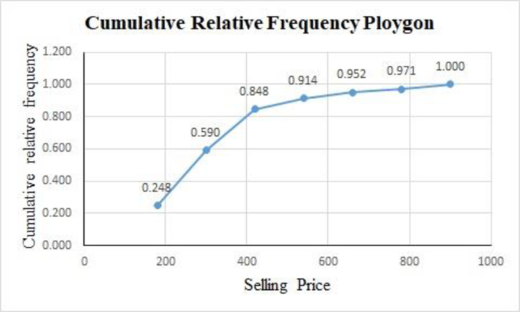
There are 50% of the homes sold approximately less than $254,000.
The top 10% of homes are sold for at least $520,000.
There are 59% of homes sold for less than $300,000.
Explanation of Solution
For the given data set, the cumulative relative frequency table with midpoints of classes is obtained as follows:
|
Selling price (1,000’s) | Midpoint |
Cumulative frequency |
Relative cumulative frequency |
| 120-240 | 26 | ||
| 240-360 | 62 | ||
| 360-480 | 89 | ||
| 480-600 | 96 | ||
| 600-720 | 100 | ||
| 720-840 | 102 | ||
| 840-960 | 105 |
The cumulative relative frequency polygon for the given data can be drawn using EXCEL.
Step-by-step procedure to obtain the frequency polygon using EXCEL is as follows:
- Enter the column of midpoints along with the cumulative relative frequency column.
- Select the total data range with labels.
- Go to Insert > Charts > line chart.
- Select the appropriate line chart.
- Click OK.
From the above cumulative relative frequency polygon, 50% of the homes are sold approximately less than $254,000.
The top 10% of homes are sold for at least $520,000.
There are 59% of homes sold for less than $300,000.
d.
Create a bar chart for the number of bedrooms for the variable bedrooms.
Answer to Problem 51DA
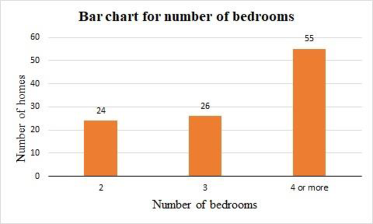
The bar chart for the number of bedrooms for the variable bedrooms is as follows:
Explanation of Solution
For the variable bedrooms, the frequency table is obtained as follows:
|
Number of bedrooms | Frequency |
| 2 | 24 |
| 3 | 26 |
| 4 or more | 55 |
| Total | 105 |
The bar chart for the given data can be drawn using EXCEL.
Step-by-step procedure to obtain the bar chart using EXCEL is as follows:
- Enter the column of bedrooms along with the frequency column.
- Select the total data range with labels.
- Go to Insert > Charts > bar chart.
- Select the appropriate bar chart.
- Click OK.
From the above bar chart, the highest frequency occurred in the last category, the shape of the distribution is negatively skewed.
Want to see more full solutions like this?
Chapter 2 Solutions
EBK STATISTICAL TECHNIQUES IN BUSINESS


- 38. Possible values of X, the number of components in a system submitted for repair that must be replaced, are 1, 2, 3, and 4 with corresponding probabilities .15, .35, .35, and .15, respectively. a. Calculate E(X) and then E(5 - X).b. Would the repair facility be better off charging a flat fee of $75 or else the amount $[150/(5 - X)]? [Note: It is not generally true that E(c/Y) = c/E(Y).]arrow_forward74. The proportions of blood phenotypes in the U.S. popula- tion are as follows:A B AB O .40 .11 .04 .45 Assuming that the phenotypes of two randomly selected individuals are independent of one another, what is the probability that both phenotypes are O? What is the probability that the phenotypes of two randomly selected individuals match?arrow_forward53. A certain shop repairs both audio and video compo- nents. Let A denote the event that the next component brought in for repair is an audio component, and let B be the event that the next component is a compact disc player (so the event B is contained in A). Suppose that P(A) = .6 and P(B) = .05. What is P(BA)?arrow_forward
- 26. A certain system can experience three different types of defects. Let A;(i = 1,2,3) denote the event that the sys- tem has a defect of type i. Suppose thatP(A1) = .12 P(A) = .07 P(A) = .05P(A, U A2) = .13P(A, U A3) = .14P(A2 U A3) = .10P(A, A2 A3) = .011Rshelfa. What is the probability that the system does not havea type 1 defect?b. What is the probability that the system has both type 1 and type 2 defects?c. What is the probability that the system has both type 1 and type 2 defects but not a type 3 defect? d. What is the probability that the system has at most two of these defects?arrow_forwardThe following are suggested designs for group sequential studies. Using PROCSEQDESIGN, provide the following for the design O’Brien Fleming and Pocock.• The critical boundary values for each analysis of the data• The expected sample sizes at each interim analysisAssume the standardized Z score method for calculating boundaries.Investigators are evaluating the success rate of a novel drug for treating a certain type ofbacterial wound infection. Since no existing treatment exists, they have planned a one-armstudy. They wish to test whether the success rate of the drug is better than 50%, whichthey have defined as the null success rate. Preliminary testing has estimated the successrate of the drug at 55%. The investigators are eager to get the drug into production andwould like to plan for 9 interim analyses (10 analyzes in total) of the data. Assume thesignificance level is 5% and power is 90%.Besides, draw a combined boundary plot (OBF, POC, and HP)arrow_forwardPlease provide the solution for the attached image in detailed.arrow_forward
- 20 km, because GISS Worksheet 10 Jesse runs a small business selling and delivering mealie meal to the spaza shops. He charges a fixed rate of R80, 00 for delivery and then R15, 50 for each packet of mealle meal he delivers. The table below helps him to calculate what to charge his customers. 10 20 30 40 50 Packets of mealie meal (m) Total costs in Rands 80 235 390 545 700 855 (c) 10.1. Define the following terms: 10.1.1. Independent Variables 10.1.2. Dependent Variables 10.2. 10.3. 10.4. 10.5. Determine the independent and dependent variables. Are the variables in this scenario discrete or continuous values? Explain What shape do you expect the graph to be? Why? Draw a graph on the graph provided to represent the information in the table above. TOTAL COST OF PACKETS OF MEALIE MEAL 900 800 700 600 COST (R) 500 400 300 200 100 0 10 20 30 40 60 NUMBER OF PACKETS OF MEALIE MEALarrow_forwardLet X be a random variable with support SX = {−3, 0.5, 3, −2.5, 3.5}. Part ofits probability mass function (PMF) is given bypX(−3) = 0.15, pX(−2.5) = 0.3, pX(3) = 0.2, pX(3.5) = 0.15.(a) Find pX(0.5).(b) Find the cumulative distribution function (CDF), FX(x), of X.1(c) Sketch the graph of FX(x).arrow_forwardA well-known company predominantly makes flat pack furniture for students. Variability with the automated machinery means the wood components are cut with a standard deviation in length of 0.45 mm. After they are cut the components are measured. If their length is more than 1.2 mm from the required length, the components are rejected. a) Calculate the percentage of components that get rejected. b) In a manufacturing run of 1000 units, how many are expected to be rejected? c) The company wishes to install more accurate equipment in order to reduce the rejection rate by one-half, using the same ±1.2mm rejection criterion. Calculate the maximum acceptable standard deviation of the new process.arrow_forward
- 5. Let X and Y be independent random variables and let the superscripts denote symmetrization (recall Sect. 3.6). Show that (X + Y) X+ys.arrow_forward8. Suppose that the moments of the random variable X are constant, that is, suppose that EX" =c for all n ≥ 1, for some constant c. Find the distribution of X.arrow_forward9. The concentration function of a random variable X is defined as Qx(h) = sup P(x ≤ X ≤x+h), h>0. Show that, if X and Y are independent random variables, then Qx+y (h) min{Qx(h). Qr (h)).arrow_forward
 Holt Mcdougal Larson Pre-algebra: Student Edition...AlgebraISBN:9780547587776Author:HOLT MCDOUGALPublisher:HOLT MCDOUGAL
 Glencoe Algebra 1, Student Edition, 9780079039897...AlgebraISBN:9780079039897Author:CarterPublisher:McGraw Hill
 Big Ideas Math A Bridge To Success Algebra 1: Stu...AlgebraISBN:9781680331141Author:HOUGHTON MIFFLIN HARCOURTPublisher:Houghton Mifflin Harcourt
 Functions and Change: A Modeling Approach to Coll...AlgebraISBN:9781337111348Author:Bruce Crauder, Benny Evans, Alan NoellPublisher:Cengage Learning