Videos
Refer to the Real Estate data, which reports information on homes sold in the Goodyear, Arizona, area during the last year. Select an appropriate class interval and organize the selling prices into a frequency distribution. Write a brief report summarizing your findings. Be sure to answer the following questions in your report.
- a. Around what values do the data tend to cluster?
- b. Based on the frequency distribution, what is the typical selling price in the first class? What is the typical selling price in the last class?
- c. Draw a cumulative frequency distribution. How many homes sold for less than $200,000? Estimate the percent of the homes that sold for more than $220,000. What percent of the homes sold for less than $125,000?
- d. Refer to the variable regarding the townships. Draw a bar chart showing the number of homes sold in each township. Are there any differences or is the number of homes sold about the same in each township?
a.
Find an appropriate class interval.
Create a frequency distribution for the selling prices and explain the results.
Find the values of price that the data tend to cluster.
Answer to Problem 51DE
The data tend to cluster between 180 (in $000) and 250 (in $000).
Explanation of Solution
Here, the data set consists of 105 observations. The value of k can be obtained as follows:
Here,
Therefore, the number of classes for the given data set is 7.
From the real estate data, the minimum and maximum values of selling price are 125 (in $000) and 345.3 (in $000), respectively.
The formula for the class interval is given as follows:
Where, i is the class interval and k is the number of classes.
Therefore, the class interval for the given data can be obtained as follows:
In practice, the class interval size is usually rounded up to some convenient number. Therefore, the reasonable class interval is 35.
Frequency distribution:
Frequency table is a collection of mutually exclusive and exhaustive classes, which shows the number of observations in each class.
Since the minimum value is 125 and the class interval is 35, the first class would be 110-145. Here, the first one is preferred as the first class of the frequency distribution. The frequency distribution for selling price is constructed as follows:
|
Selling price (1,000’s) | Frequency |
Cumulative frequency |
| 110-145 | 3 | 3 |
| 145-180 | 19 | |
| 180-215 | 31 | |
| 215-250 | 25 | |
| 250-285 | 14 | |
| 285-320 | 10 | |
| 320-355 | 3 | |
| Total | 105 |
From the above table, it is clear that maximum values of frequency are obtained for the intervals 180-215 and 215-250. Their corresponding frequencies are 31 and 25, respectively.
That is, 53%
b.
Find the typical selling in the first class.
Find the typical selling in the last class.
Answer to Problem 51DE
The typical selling price of the first class is 127.5 (in $000).
The typical selling price of the last class is 337.5 (in $000).
Explanation of Solution
The lower and upper limits of the first class are 110 and 145, respectively.
The typical selling price of the first class is calculated as follows:
Thus, the typical selling price of the first class is 127.5 (in $000).
The lower and upper limits of the last class are 355 and 320, respectively.
The typical selling price of the last class is calculated as follows:
Thus, the typical selling price of the last class is 337.5 (in $000).
c.
Plot the cumulative frequency distribution.
Find the number of homes sold for less than $200,000.
Find the percent of homes sold for more than $220,000.
Find the percentage of homes sold for less than $125,000.
Answer to Problem 51DE
The plot of the cumulative frequency distribution for the given data is as follows:
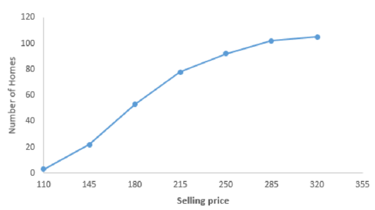
The number of homes sold for less than $200,000 is 42.
The percent of homes sold for more than $200,000 46.7.
The percentage of homes sold for less than $125,000 is 0%.
Explanation of Solution
Step-by-step procedure to obtain the plot using the EXCEL is as follows:
- Select the data range.
- Go to Insert > Charts > line chart.
- Select the Scatter with Straight Lines and Markers under Charts.
Thus, the plot is obtained.
Step-by-step procedure to find the number of homes sold for less than $200,000:
- Select Insert > PivotTable.
- In Table/Range, select the data range.
- Move Selling Price to Rows.
- Again move Selling Price to ∑Values.
- Right click on any data in Row Labels.
- Select Group.
- In Grouping, enter 100 in Starting at, 360 in Ending at, and enter 20 in By.
Output is obtained as follows:
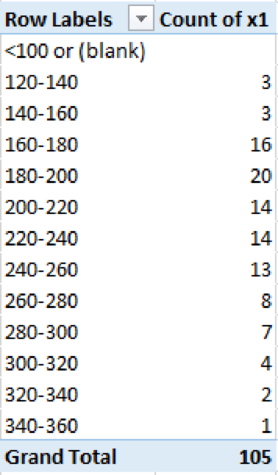
From the above output, the number of homes sold for less than $200,000 is 42
The percent of homes that are sold for more than $220,000 is 46.7%
In the data set, the minimum value is 125. Therefore, no homes are sold for less than $125,000. Therefore, the percentage of homes sold for less than $125,000 is 0%.
d.
Create a bar chart for the number of homes sold in each township.
Explain whether the number of homes sold is about the same in each township.
Answer to Problem 51DE
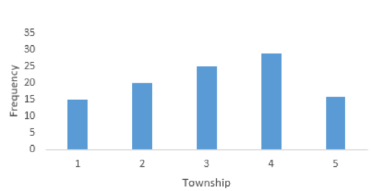
The bar chart that represents the number of homes sold in each township is as follows:
Explanation of Solution
For the variable Township, the frequency table is obtained as follows:
| Township | Frequency |
| 1 | 15 |
| 2 | 20 |
| 3 | 25 |
| 4 | 29 |
| 5 | 16 |
The bar chart for the given data can be drawn using EXCEL.
Step-by-step procedure to obtain the bar chart using EXCEL:
- Enter the column of township along with their frequency column.
- Select the total data range with labels.
- Go to Insert > Charts > bar chart.
- Select the appropriate bar chart.
- Click OK.
Thus, the bar chart is obtained.
From the above bar chart, the highest frequency occurred for townships 3 and 4 and the lowest frequency occurred for townships 1 and 5. Thus, the number of homes sold is not about the same in each township.
Want to see more full solutions like this?
Chapter 2 Solutions
Statistical Techniques in Business and Economics


- Question 2: When John started his first job, his first end-of-year salary was $82,500. In the following years, he received salary raises as shown in the following table. Fill the Table: Fill the following table showing his end-of-year salary for each year. I have already provided the end-of-year salaries for the first three years. Calculate the end-of-year salaries for the remaining years using Excel. (If you Excel answer for the top 3 cells is not the same as the one in the following table, your formula / approach is incorrect) (2 points) Geometric Mean of Salary Raises: Calculate the geometric mean of the salary raises using the percentage figures provided in the second column named “% Raise”. (The geometric mean for this calculation should be nearly identical to the arithmetic mean. If your answer deviates significantly from the mean, it's likely incorrect. 2 points) Starting salary % Raise Raise Salary after raise 75000 10% 7500 82500 82500 4% 3300…arrow_forwardI need help with this problem and an explanation of the solution for the image described below. (Statistics: Engineering Probabilities)arrow_forwardI need help with this problem and an explanation of the solution for the image described below. (Statistics: Engineering Probabilities)arrow_forward
- 310015 K Question 9, 5.2.28-T Part 1 of 4 HW Score: 85.96%, 49 of 57 points Points: 1 Save of 6 Based on a poll, among adults who regret getting tattoos, 28% say that they were too young when they got their tattoos. Assume that six adults who regret getting tattoos are randomly selected, and find the indicated probability. Complete parts (a) through (d) below. a. Find the probability that none of the selected adults say that they were too young to get tattoos. 0.0520 (Round to four decimal places as needed.) Clear all Final check Feb 7 12:47 US Oarrow_forwardhow could the bar graph have been organized differently to make it easier to compare opinion changes within political partiesarrow_forwardDraw a picture of a normal distribution with mean 70 and standard deviation 5.arrow_forward
- What do you guess are the standard deviations of the two distributions in the previous example problem?arrow_forwardPlease answer the questionsarrow_forward30. An individual who has automobile insurance from a certain company is randomly selected. Let Y be the num- ber of moving violations for which the individual was cited during the last 3 years. The pmf of Y isy | 1 2 4 8 16p(y) | .05 .10 .35 .40 .10 a.Compute E(Y).b. Suppose an individual with Y violations incurs a surcharge of $100Y^2. Calculate the expected amount of the surcharge.arrow_forward
- 24. An insurance company offers its policyholders a num- ber of different premium payment options. For a ran- domly selected policyholder, let X = the number of months between successive payments. The cdf of X is as follows: F(x)=0.00 : x < 10.30 : 1≤x<30.40 : 3≤ x < 40.45 : 4≤ x <60.60 : 6≤ x < 121.00 : 12≤ x a. What is the pmf of X?b. Using just the cdf, compute P(3≤ X ≤6) and P(4≤ X).arrow_forward59. At a certain gas station, 40% of the customers use regular gas (A1), 35% use plus gas (A2), and 25% use premium (A3). Of those customers using regular gas, only 30% fill their tanks (event B). Of those customers using plus, 60% fill their tanks, whereas of those using premium, 50% fill their tanks.a. What is the probability that the next customer will request plus gas and fill the tank (A2 B)?b. What is the probability that the next customer fills the tank?c. If the next customer fills the tank, what is the probability that regular gas is requested? Plus? Premium?arrow_forward38. Possible values of X, the number of components in a system submitted for repair that must be replaced, are 1, 2, 3, and 4 with corresponding probabilities .15, .35, .35, and .15, respectively. a. Calculate E(X) and then E(5 - X).b. Would the repair facility be better off charging a flat fee of $75 or else the amount $[150/(5 - X)]? [Note: It is not generally true that E(c/Y) = c/E(Y).]arrow_forward
 Big Ideas Math A Bridge To Success Algebra 1: Stu...AlgebraISBN:9781680331141Author:HOUGHTON MIFFLIN HARCOURTPublisher:Houghton Mifflin Harcourt
 Holt Mcdougal Larson Pre-algebra: Student Edition...AlgebraISBN:9780547587776Author:HOLT MCDOUGALPublisher:HOLT MCDOUGAL
 Glencoe Algebra 1, Student Edition, 9780079039897...AlgebraISBN:9780079039897Author:CarterPublisher:McGraw Hill
 Functions and Change: A Modeling Approach to Coll...AlgebraISBN:9781337111348Author:Bruce Crauder, Benny Evans, Alan NoellPublisher:Cengage Learning