Concept explainers
Videos
Compare the frequency histograms of men’s winning scores and women’s winning scores for different classes of 5, 7, and 10 and comment on general shape of the histograms.
Answer to Problem 2UT
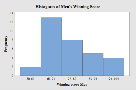
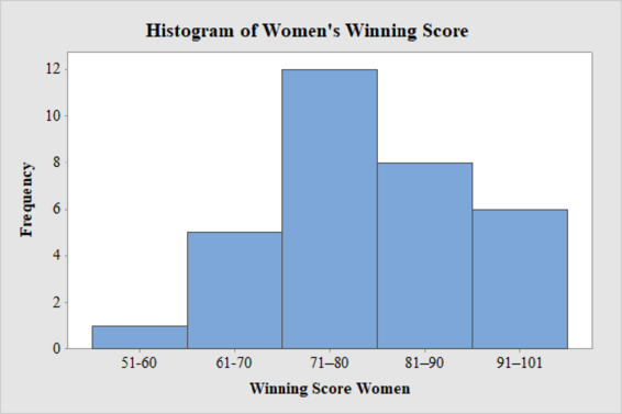
The frequency histogram for the data on men’s and women’s winning scores with five classes is shown below:
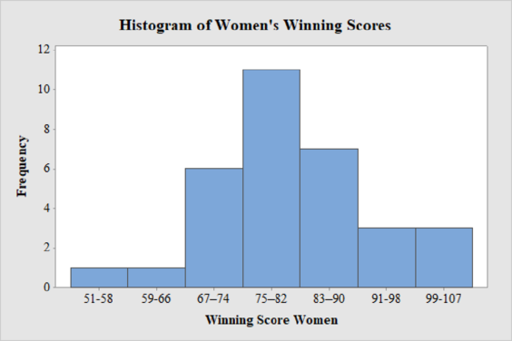
The frequency histogram for the data on men’s and women’s winning scores with seven classes is shown below:
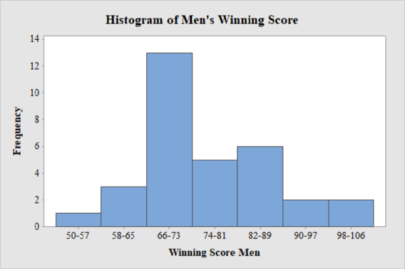
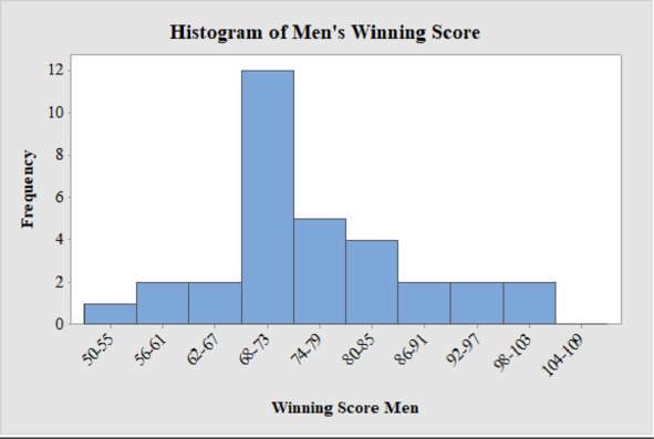
The frequency histogram for the data on men’s winning scores with ten classes is shown below:
The best choice for number of classes is seven.
Explanation of Solution
Calculation:
Class limits:
Class limits are the maximum and minimum values in the class interval.
Class Boundaries:
A class boundary is the midpoint between the upper limit of one class and the lower limit of the next class where the upper limit of the preceding class interval and the lower limit of the next class interval will be equal. The upper class boundary is calculated by adding 0.5 to the upper class limit and the lower class boundary is calculated by subtracting 0.5 from the lower class limit.
Frequency:
Frequency is the number of data points that fall under each class.
Men’s Winning Score with five classes:
From the given data set, the largest data point is 101 and the smallest data point is 50.
Class Width:
The class width is calculated as follows:
The class width is 11. Hence, the lower class limit for the second class 61 is calculated by adding 11 to 50. Following this pattern, all the lower class limits are established. Then, the upper class limits are calculated.
The frequency distribution table is given below:
| Class Limits | Class Boundaries | Frequency |
| 50-60 | 49.5-60.5 | 2 |
| 61-71 | 60.5-71.5 | 13 |
| 72–82 | 71.5–82.5 | 8 |
| 83–93 | 82.5–93.5 | 5 |
| 94–104 | 93.5–104.5 | 4 |
Step-by-step procedure to draw the histogram using MINITAB software:
- Choose Graph > Bar Chart.
- From Bars represent, choose Values from a table.
- Under One column of values, choose Simple. Click OK.
- In Graph variables, enter the column of Frequency.
- In Categorical variables, enter the column of Winning Score Men.
- Click OK.
Thus, the histogram for men’s winning score with five classes is obtained.
Men’s Winning Score with seven classes:
From the given data set, the largest data point is 101 and the smallest data point is 50.
Class Width:
The class width is calculated as follows:
The class width is 8. Hence, the lower class limit for the second class 58 is calculated by adding 8 to 50. Following this pattern, all the lower class limits are established. Then, the upper class limits are calculated.
The frequency distribution table is given below:
| Class Limits | Class Boundaries | Frequency |
| 50-57 | 49.5-57.5 | 1 |
| 58-65 | 57.5-65.5 | 3 |
| 66-73 | 65.5-73.5 | 13 |
| 74-81 | 73.5-81.5 | 5 |
| 82-89 | 81.5-89.5 | 6 |
| 90-97 | 89.5-97.5 | 2 |
| 98-106 | 97.5-106.5 | 2 |
Step-by-step procedure to draw the histogram using MINITAB software:
- Choose Graph > Bar Chart.
- From Bars represent, choose Values from a table.
- Under One column of values, choose Simple. Click OK.
- In Graph variables, enter the column of Frequency.
- In Categorical variables, enter the column of Winning Score Men.
- Click OK.
Thus, the histogram for men’s winning score with seven classes is obtained.
Men’s Winning Score with ten classes:
From the given data set, the largest data point is 101 and the smallest data point is 50.
Class Width:
The class width is calculated as follows:
The class width is 6. Hence, the lower class limit for the second class 56 is calculated by adding 6 to 50. Following this pattern, all the lower class limits are established. Then, the upper class limits are calculated.
The frequency distribution table is given below:
| Class Limits | Class Boundaries | Frequency |
| 50-55 | 49.5-55.5 | 1 |
| 56-61 | 55.5-61.5 | 2 |
| 62-67 | 61.5-67.5 | 2 |
| 68-73 | 67.5-73.5 | 12 |
| 74-79 | 73.5-79.5 | 5 |
| 80-85 | 79.5-85.5 | 4 |
| 86-91 | 85.5-91.5 | 2 |
| 92-97 | 91.5-97.5 | 2 |
| 98-103 | 97.5-103.5 | 2 |
| 104-109 | 103.5-109.5 | 0 |
Step-by-step procedure to draw the histogram using MINITAB software:
- Choose Graph > Bar Chart.
- From Bars represent, choose Values from a table.
- Under One column of values, choose Simple. Click OK.
- In Graph variables, enter the column of Frequency.
- In Categorical variables, enter the column of Winning Score Men.
- Click OK.
Thus, the histogram for men’s winning score with ten classes is obtained.
Women’s Winning Score with five classes:
From the given data set, the largest data point is 101 and the smallest data point is 51.
Class Width:
The class width is calculated as follows:
The class width is 10. Hence, the lower class limit for the second class 61 is calculated by adding 10 to 51. Following this pattern, all the lower class limits are established. Then, the upper class limits are calculated.
The frequency distribution table is given below:
| Class Limits | Class Boundaries | Frequency |
| 51-60 | 50.5-60.5 | 1 |
| 61-70 | 60.5-70.5 | 5 |
| 71–80 | 70.5–80.5 | 12 |
| 81–90 | 80.5–90.5 | 8 |
| 91–101 | 90.5–101.5 | 6 |
Step-by-step procedure to draw the histogram using MINITAB software:
- Choose Graph > Bar Chart.
- From Bars represent, choose Values from a table.
- Under One column of values, choose Simple. Click OK.
- In Graph variables, enter the column of Frequency.
- In Categorical variables, enter the column of Winning Score Women.
- Click OK.
Thus, the histogram for women’s winning score with five classes is obtained.
Women’s Winning Score with seven classes:
From the given data set, the largest data point is 101 and the smallest data point is 51.
Class Width:
The class width is calculated as follows:
The class width is 8. Hence, the lower class limit for the second class 59 is calculated by adding 8 to 51. Following this pattern, all the lower class limits are established. Then, the upper class limits are calculated.
The frequency distribution table is given below:
| Class Limits | Class Boundaries | Frequency |
| 51-58 | 50.5-58.5 | 1 |
| 59-66 | 58.5-66.5 | 1 |
| 67–74 | 66.5–74.5 | 6 |
| 75–82 | 74.5–82.5 | 11 |
| 83–90 | 82.5–90.5 | 7 |
| 91-98 | 90.5-98.5 | 3 |
| 99-107 | 98.5-107.5 | 3 |
Step-by-step procedure to draw the histogram using MINITAB software:
- Choose Graph > Bar Chart.
- From Bars represent, choose Values from a table.
- Under One column of values, choose Simple. Click OK.
- In Graph variables, enter the column of Frequency.
- In Categorical variables, enter the column of Winning Score Women.
- Click OK.
Thus, the histogram for women’s winning score with seven classes is obtained.
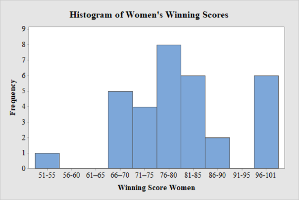
Women’s Winning Score with ten classes:
From the given data set, the largest data point is 101 and the smallest data point is 51.
Class Width:
The class width is calculated as follows:
The class width is 5. Hence, the lower class limit for the second class 56 is calculated by adding 5 to 51. Following this pattern, all the lower class limits are established. Then, the upper class limits are calculated.
The frequency distribution table is given below:
| Class Limits | Class Boundaries | Frequency |
| 51-55 | 50.5-55.5 | 1 |
| 56-60 | 55.5-60.5 | 0 |
| 61–65 | 60.5–65.5 | 0 |
| 66–70 | 65.5–70.5 | 5 |
| 71–75 | 70.5–75.5 | 4 |
| 76-80 | 75.5-80.5 | 8 |
| 81-85 | 80.5-85.5 | 6 |
| 86-90 | 85.5-90.5 | 2 |
| 91-95 | 90.5-95.5 | 0 |
| 96-101 | 95.5-101.5 | 6 |
Step-by-step procedure to draw the histogram using MINITAB software:
- Choose Graph > Bar Chart.
- From Bars represent, choose Values from a table.
- Under One column of values, choose Simple. Click OK.
- In Graph variables, enter the column of Frequency.
- In Categorical variables, enter the column of Winning Score Women.
- Click OK.
Thus, the histogram for women’s winning score with ten classes is obtained.
Comparison of men’s and women’s winning score:
Five classes:
From the histogram on men’s and women’s winning scores with five classes, the following can be observed:
- The data values of men’s winning scores fall within 50 and 101, and the data values of women’s winning scores range between 51 and 101.
- The shape of distribution of men’s winning scores is skewed to the right and there are no unusual observations in the data as not even one data point is far from the overall bulk of data.
- The shape of distribution of women’s winning scores is approximately mound-shaped and there are no outliers.
Seven classes:
From the histogram on men’s and women’s winning scores with seven classes, the following can be observed:
- The data values of men’s winning scores fall within 50 and 101, and the data values of women’s winning scores range between 51 and 101.
- The shape of distribution of men’s winning scores is almost skewed to the right and there are no unusual observations in the data as not even one data point is far from the overall bulk of data.
- The shape of distribution of women’s winning scores is approximately mound-shaped and there are no outliers.
Ten classes:
From the histogram on men’s and women’s winning scores with seven classes, the following can be observed:
- The data values of men’s winning scores fall within 50 and 101 and the data values of women’s winning scores range between 51 and 101.
- The shape of distribution of men’s winning scores is slightly skewed to the right and there are no unusual observations in the data as not even one data point is far from the overall bulk of data. There is only one peak in the distribution.
- The shape of distribution of women’s winning scores is skewed to the left and there is an unusual observation in the data as there are few observations that fall away from the overall bulk of data.
Want to see more full solutions like this?
Chapter 2 Solutions
Bundle: Understandable Statistics: Concepts And Methods, 12th + Jmp Printed Access Card For Peck's Statistics + Webassign Printed Access Card For ... And Methods, 12th Edition, Single-term


- High Cholesterol: A group of eight individuals with high cholesterol levels were given a new drug that was designed to lower cholesterol levels. Cholesterol levels, in milligrams per deciliter, were measured before and after treatment for each individual, with the following results: Individual Before 1 2 3 4 5 6 7 8 237 282 278 297 243 228 298 269 After 200 208 178 212 174 201 189 185 Part: 0/2 Part 1 of 2 (a) Construct a 99.9% confidence interval for the mean reduction in cholesterol level. Let a represent the cholesterol level before treatment minus the cholesterol level after. Use tables to find the critical value and round the answers to at least one decimal place.arrow_forwardI worked out the answers for most of this, and provided the answers in the tables that follow. But for the total cost table, I need help working out the values for 10%, 11%, and 12%. A pharmaceutical company produces the drug NasaMist from four chemicals. Today, the company must produce 1000 pounds of the drug. The three active ingredients in NasaMist are A, B, and C. By weight, at least 8% of NasaMist must consist of A, at least 4% of B, and at least 2% of C. The cost per pound of each chemical and the amount of each active ingredient in one pound of each chemical are given in the data at the bottom. It is necessary that at least 100 pounds of chemical 2 and at least 450 pounds of chemical 3 be used. a. Determine the cheapest way of producing today’s batch of NasaMist. If needed, round your answers to one decimal digit. Production plan Weight (lbs) Chemical 1 257.1 Chemical 2 100 Chemical 3 450 Chemical 4 192.9 b. Use SolverTable to see how much the percentage of…arrow_forwardAt the beginning of year 1, you have $10,000. Investments A and B are available; their cash flows per dollars invested are shown in the table below. Assume that any money not invested in A or B earns interest at an annual rate of 2%. a. What is the maximized amount of cash on hand at the beginning of year 4.$ ___________ A B Time 0 -$1.00 $0.00 Time 1 $0.20 -$1.00 Time 2 $1.50 $0.00 Time 3 $0.00 $1.90arrow_forward
- For each of the time series, construct a line chart of the data and identify the characteristics of the time series (that is, random, stationary, trend, seasonal, or cyclical). Year Month Rate (%)2009 Mar 8.72009 Apr 9.02009 May 9.42009 Jun 9.52009 Jul 9.52009 Aug 9.62009 Sep 9.82009 Oct 10.02009 Nov 9.92009 Dec 9.92010 Jan 9.82010 Feb 9.82010 Mar 9.92010 Apr 9.92010 May 9.62010 Jun 9.42010 Jul 9.52010 Aug 9.52010 Sep 9.52010 Oct 9.52010 Nov 9.82010 Dec 9.32011 Jan 9.12011 Feb 9.02011 Mar 8.92011 Apr 9.02011 May 9.02011 Jun 9.12011 Jul 9.02011 Aug 9.02011 Sep 9.02011 Oct 8.92011 Nov 8.62011 Dec 8.52012 Jan 8.32012 Feb 8.32012 Mar 8.22012 Apr 8.12012 May 8.22012 Jun 8.22012 Jul 8.22012 Aug 8.12012 Sep 7.82012 Oct…arrow_forwardFor each of the time series, construct a line chart of the data and identify the characteristics of the time series (that is, random, stationary, trend, seasonal, or cyclical). Date IBM9/7/2010 $125.959/8/2010 $126.089/9/2010 $126.369/10/2010 $127.999/13/2010 $129.619/14/2010 $128.859/15/2010 $129.439/16/2010 $129.679/17/2010 $130.199/20/2010 $131.79 a. Construct a line chart of the closing stock prices data. Choose the correct chart below.arrow_forwardFor each of the time series, construct a line chart of the data and identify the characteristics of the time series (that is, random, stationary, trend, seasonal, or cyclical) Date IBM9/7/2010 $125.959/8/2010 $126.089/9/2010 $126.369/10/2010 $127.999/13/2010 $129.619/14/2010 $128.859/15/2010 $129.439/16/2010 $129.679/17/2010 $130.199/20/2010 $131.79arrow_forward
- 1. A consumer group claims that the mean annual consumption of cheddar cheese by a person in the United States is at most 10.3 pounds. A random sample of 100 people in the United States has a mean annual cheddar cheese consumption of 9.9 pounds. Assume the population standard deviation is 2.1 pounds. At a = 0.05, can you reject the claim? (Adapted from U.S. Department of Agriculture) State the hypotheses: Calculate the test statistic: Calculate the P-value: Conclusion (reject or fail to reject Ho): 2. The CEO of a manufacturing facility claims that the mean workday of the company's assembly line employees is less than 8.5 hours. A random sample of 25 of the company's assembly line employees has a mean workday of 8.2 hours. Assume the population standard deviation is 0.5 hour and the population is normally distributed. At a = 0.01, test the CEO's claim. State the hypotheses: Calculate the test statistic: Calculate the P-value: Conclusion (reject or fail to reject Ho): Statisticsarrow_forward21. find the mean. and variance of the following: Ⓒ x(t) = Ut +V, and V indepriv. s.t U.VN NL0, 63). X(t) = t² + Ut +V, U and V incepires have N (0,8) Ut ①xt = e UNN (0162) ~ X+ = UCOSTE, UNNL0, 62) SU, Oct ⑤Xt= 7 where U. Vindp.rus +> ½ have NL, 62). ⑥Xn = ΣY, 41, 42, 43, ... Yn vandom sample K=1 Text with mean zen and variance 6arrow_forwardA psychology researcher conducted a Chi-Square Test of Independence to examine whether there is a relationship between college students’ year in school (Freshman, Sophomore, Junior, Senior) and their preferred coping strategy for academic stress (Problem-Focused, Emotion-Focused, Avoidance). The test yielded the following result: image.png Interpret the results of this analysis. In your response, clearly explain: Whether the result is statistically significant and why. What this means about the relationship between year in school and coping strategy. What the researcher should conclude based on these findings.arrow_forward
- A school counselor is conducting a research study to examine whether there is a relationship between the number of times teenagers report vaping per week and their academic performance, measured by GPA. The counselor collects data from a sample of high school students. Write the null and alternative hypotheses for this study. Clearly state your hypotheses in terms of the correlation between vaping frequency and academic performance. EditViewInsertFormatToolsTable 12pt Paragrapharrow_forwardA smallish urn contains 25 small plastic bunnies – 7 of which are pink and 18 of which are white. 10 bunnies are drawn from the urn at random with replacement, and X is the number of pink bunnies that are drawn. (a) P(X = 5) ≈ (b) P(X<6) ≈ The Whoville small urn contains 100 marbles – 60 blue and 40 orange. The Grinch sneaks in one night and grabs a simple random sample (without replacement) of 15 marbles. (a) The probability that the Grinch gets exactly 6 blue marbles is [ Select ] ["≈ 0.054", "≈ 0.043", "≈ 0.061"] . (b) The probability that the Grinch gets at least 7 blue marbles is [ Select ] ["≈ 0.922", "≈ 0.905", "≈ 0.893"] . (c) The probability that the Grinch gets between 8 and 12 blue marbles (inclusive) is [ Select ] ["≈ 0.801", "≈ 0.760", "≈ 0.786"] . The Whoville small urn contains 100 marbles – 60 blue and 40 orange. The Grinch sneaks in one night and grabs a simple random sample (without replacement) of 15 marbles. (a)…arrow_forwardSuppose an experiment was conducted to compare the mileage(km) per litre obtained by competing brands of petrol I,II,III. Three new Mazda, three new Toyota and three new Nissan cars were available for experimentation. During the experiment the cars would operate under same conditions in order to eliminate the effect of external variables on the distance travelled per litre on the assigned brand of petrol. The data is given as below: Brands of Petrol Mazda Toyota Nissan I 10.6 12.0 11.0 II 9.0 15.0 12.0 III 12.0 17.4 13.0 (a) Test at the 5% level of significance whether there are signi cant differences among the brands of fuels and also among the cars. [10] (b) Compute the standard error for comparing any two fuel brands means. Hence compare, at the 5% level of significance, each of fuel brands II, and III with the standard fuel brand I. [10] �arrow_forward
 Big Ideas Math A Bridge To Success Algebra 1: Stu...AlgebraISBN:9781680331141Author:HOUGHTON MIFFLIN HARCOURTPublisher:Houghton Mifflin Harcourt
 Glencoe Algebra 1, Student Edition, 9780079039897...AlgebraISBN:9780079039897Author:CarterPublisher:McGraw Hill
 Holt Mcdougal Larson Pre-algebra: Student Edition...AlgebraISBN:9780547587776Author:HOLT MCDOUGALPublisher:HOLT MCDOUGAL