Chapter 2, Problem 1UT

To determine

Create frequency histograms for the data on men’s winning scores with classes of 5, 7, and 10.

Create frequency histograms for the data on women’s winning scores with classes of 5, 7, and 10.

Identify the best choice of the number of classes and give reason.

Answer to Problem 1UT

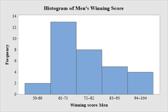
The frequency histogram for the data on men’s winning scores with five classes is shown below:

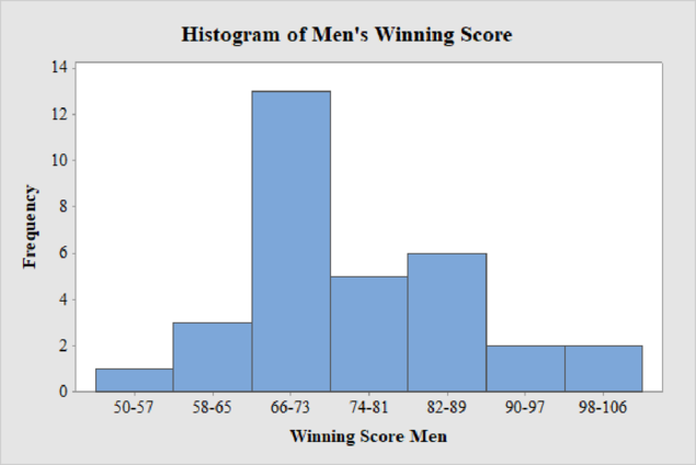
The frequency histogram for the data on men’s winning scores with seven classes is shown below:

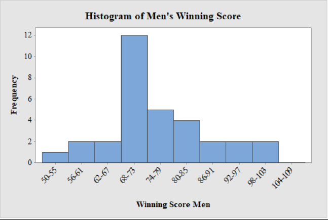
The frequency histogram for the data on men’s winning scores with ten classes is shown below:

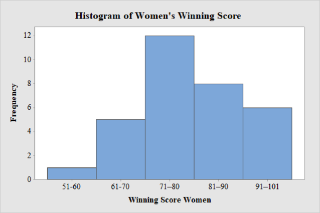
The frequency histogram for the data on women’s winning scores with five classes is shown below:

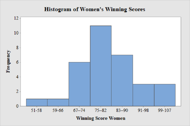
The frequency histogram for the data on women’s winning scores with seven classes is shown below:

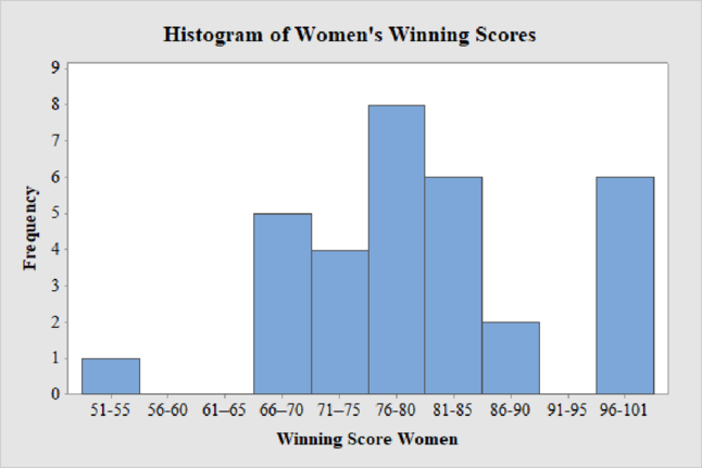
The frequency histogram for the data on women’s winning scores with ten classes is shown below:

The best choice for the number of classes is seven.

Explanation of Solution

Calculation:

Class limits:

Class limits are the maximum and minimum values in the class interval

Class Boundaries:

A class boundary is the midpoint between the upper limit of one class and the lower limit of the next class where the upper limit of the preceding class interval and the lower limit of the next class interval will be equal. The upper class boundary is calculated by adding 0.5 to the upper class limit and the lower class boundary is calculated by subtracting 0.5 from the lower class limit.

Frequency:

Frequency is the number of data points that fall under each class.

Men’s Winning Score with five classes:

From the given data set, the largest data point is 101 and the smallest data point is 50.

Class Width:

The class width is calculated as follows:

$\begin{array}{c}\text{Class width=}\frac{\left(\text{Largest data point}-\text{Smallest data point}\right)}{\text{Number of classes}}\\ \text{=}\frac{\left(101-50\right)}{5}\\ =10.2\\ \approx 11\end{array}$

The class width is 11. Hence, the lower class limit for the second class 61 is calculated by adding 11 to 50. Following this pattern, all the lower class limits are established. Then, the upper class limits are calculated.

The frequency distribution table is given below:

Class Limits	Class Boundaries	Frequency
50-60	49.5–60.5	2
61-71	60.5–71.5	13
72–82	71.5–82.5	8
83–93	82.5–93.5	5
94–104	93.5–104.5	4

Step-by-step procedure to draw the histogram using MINITAB software:

• Choose Graph > Bar Chart.
• From Bars represent, choose Values from a table.
• Under One column of values, choose Simple. Click OK.
• In Graph variables, enter the column of Frequency.
• In Categorical variables, enter the column of Winning Score Men.
• Click OK.

Thus, the histogram for men’s winning score with five classes is obtained.

Men’s Winning Score with seven classes:

From the given data set, the largest data point is 101 and the smallest data point is 50.

Class Width:

The class width is calculated as follows:

$\begin{array}{c}\text{Class width=}\frac{\left(\text{Largest data point}-\text{Smallest data point}\right)}{\text{Number of classes}}\\ \text{=}\frac{\left(101-50\right)}{7}\\ =7.28\\ \approx 8\end{array}$

The class width is 8. Hence, the lower class limit for the second class 58 is calculated by adding 8 to 50. Following this pattern, all the lower class limits are established. Then, the upper class limits are calculated.

The frequency distribution table is given below:

Class Limits	Class Boundaries	Frequency
50-57	49.5-57.5	1
58-65	57.5-65.5	3
66-73	65.5-73.5	13
74-81	73.5-81.5	5
82-89	81.5-89.5	6
90-97	89.5-97.5	2
98-106	97.5-106.5	2

Step-by-step procedure to draw the histogram using MINITAB software:

• Choose Graph > Bar Chart.
• From Bars represent, choose Values from a table.
• Under One column of values, choose Simple. Click OK.
• In Graph variables, enter the column of Frequency.
• In Categorical variables, enter the column of Winning Score Men.
• Click OK.

Thus, the histogram for men’s winning score with seven classes is obtained.

Men’s Winning Score with ten classes:

From the given data set, the largest data point is 101 and the smallest data point is 50.

Class Width:

The class width is calculated as follows:

$\begin{array}{c}\text{Class width=}\frac{\left(\text{Largest data point}-\text{Smallest data point}\right)}{\text{Number of classes}}\\ \text{=}\frac{\left(101-50\right)}{10}\\ =5.1\\ \approx 6\end{array}$

The class width is 6. Hence, the lower class limit for the second class 56 is calculated by adding 6 to 50. Following this pattern, all the lower class limits are established. Then, the upper class limits are calculated.

The frequency distribution table is given below:

Class Limits	Class Boundaries	Frequency
50-55	49.5-55.5	1
56-61	55.5-61.5	2
62-67	61.5-67.5	2
68-73	67.5-73.5	12
74-79	73.5-79.5	5
80-85	79.5-85.5	4
86-91	85.5-91.5	2
92-97	91.5-97.5	2
98-103	97.5-103.5	2
104-109	103.5-109.5	0

Step-by-step procedure to draw the histogram using MINITAB software:

• Choose Graph > Bar Chart.
• From Bars represent, choose Values from a table.
• Under One column of values, choose Simple. Click OK.
• In Graph variables, enter the column of Frequency.
• In Categorical variables, enter the column of Winning Score Men.
• Click OK.

Thus, the histogram for men’s winning score with ten classes is obtained.

Women’s Winning Score with five classes:

From the given data set, the largest data point is 101 and the smallest data point is 51.

Class Width:

The class width is calculated as follows:

$\begin{array}{c}\text{Class width=}\frac{\left(\text{Largest data point}-\text{Smallest data point}\right)}{\text{Number of classes}}\\ \text{=}\frac{\left(101-51\right)}{5}\\ =10\end{array}$

The class width is 10. Hence, the lower class limit for the second class 61 is calculated by adding 10 to 51. Following this pattern, all the lower class limits are established. Then, the upper class limits are calculated.

The frequency distribution table is given below:

Class Limits	Class Boundaries	Frequency
51-60	50.5-60.5	1
61-70	60.5-70.5	5
71–80	70.5–80.5	12
81–90	80.5–90.5	8
91–101	90.5–101.5	6

Step-by-step procedure to draw the histogram using MINITAB software:

• Choose Graph > Bar Chart.
• From Bars represent, choose Values from a table.
• Under One column of values, choose Simple. Click OK.
• In Graph variables, enter the column of Frequency.
• In Categorical variables, enter the column of Winning Score Women.
• Click OK.

Thus, the histogram for women’s winning score with five classes is obtained.

Women’s Winning Score with seven classes:

From the given data set, the largest data point is 101 and the smallest data point is 51.

Class Width:

The class width is calculated as follows:

$\begin{array}{c}\text{Class width=}\frac{\left(\text{Largest data point}-\text{Smallest data point}\right)}{\text{Number of classes}}\\ \text{=}\frac{\left(101-51\right)}{7}\\ =7.14\\ \approx 7\end{array}$

The class width is 8. Hence, the lower class limit for the second class 59 is calculated by adding 8 to 51. Following this pattern, all the lower class limits are established. Then, the upper class limits are calculated.

The frequency distribution table is given below:

Class Limits	Class Boundaries	Frequency
51-58	50.5-58.5	1
59-66	58.5-66.5	1
67–74	66.5–74.5	6
75–82	74.5–82.5	11
83–90	82.5–90.5	7
91-98	90.5-98.5	3
99-107	98.5-107.5	3

Step-by-step procedure to draw the histogram using MINITAB software:

• Choose Graph > Bar Chart.
• From Bars represent, choose Values from a table.
• Under One column of values, choose Simple. Click OK.
• In Graph variables, enter the column of Frequency.
• In Categorical variables, enter the column of Winning Score Women.
• Click OK.

Thus, the histogram for women’s winning score with seven classes is obtained.

Women’s Winning Score with ten classes:

From the given data set, the largest data point is 101 and the smallest data point is 51.

Class Width:

The class width is calculated as follows:

$\begin{array}{c}\text{Class width=}\frac{\left(\text{Largest data point}-\text{Smallest data point}\right)}{\text{Number of classes}}\\ \text{=}\frac{\left(101-51\right)}{10}\\ =5\end{array}$

The class width is 5. Hence, the lower class limit for the second class 56 is calculated by adding 5 to 51. Following this pattern, all the lower class limits are established. Then, the upper class limits are calculated.

The frequency distribution table is given below:

Class Limits	Class Boundaries	Frequency
51-55	50.5–55.5	1
56-60	55.5–60.5	0
61–65	60.5–65.5	0
66–70	65.5–70.5	5
71–75	70.5–75.5	4
76-80	75.5-80.5	8
81-85	80.5-85.5	6
86-90	85.5-90.5	2
91-95	90.5-95.5	0
96-101	95.5-101.5	6

Step-by-step procedure to draw the histogram using MINITAB software:

• Choose Graph > Bar Chart.
• From Bars represent, choose Values from a table.
• Under One column of values, choose Simple. Click OK.
• In Graph variables, enter the column of Frequency.
• In Categorical variables, enter the column of Winning Score Women.
• Click OK.

Thus, the histogram for women’s winning score with ten classes is obtained.

Best Choice of Number of classes:

From the Histograms of men and women winning scores for three different classes 5, 7 and 10, it can be observed that the histogram with seven numbers of classes is the best choice as the distribution of both men’s and women’s winning scores are approximately mound-shaped or symmetric with a single peak without any outliers.