Videos
(a)
To find: The marginal total of the provided data to add them in the table.
(a)
Answer to Problem 153E
Solution: The obtained marginal totals are shown in the below table.
Field of study |
Canada |
France |
Germany |
Italy |
Japan |
UK |
US |
Total` |
SsBL |
64 |
153 |
66 |
125 |
250 |
152 |
878 |
1688 |
SME |
35 |
111 |
66 |
80 |
136 |
128 |
355 |
911 |
AH |
27 |
74 |
33 |
42 |
123 |
105 |
397 |
801 |
Ed |
20 |
45 |
18 |
16 |
39 |
14 |
167 |
319 |
Other |
30 |
289 |
35 |
58 |
97 |
76 |
272 |
857 |
Total |
176 |
672 |
218 |
321 |
645 |
475 |
2069 |
4576 |
Explanation of Solution
Calculation: To obtain the marginal totals, below steps are followed in the Minitab software.
Step 1: Enter the data in Minitab worksheet.
Step 2: Go to Stat > Tables >
Step 3: Select “Field” in “For rows” and select “Country” in “For columns”. And select “Count” in “Frequencies are in”.
Step 4: Select the option “Counts” under the “Categorical Variables”.
Step 5: Click OK twice.
The totals are obtained as the Minitab output. The obtained marginal totals are shown in the below table.
Field of study |
Canada |
France |
Germany |
Italy |
Japan |
UK |
US |
Total |
SsBL |
64 |
153 |
66 |
125 |
250 |
152 |
878 |
1688 |
SME |
35 |
111 |
66 |
80 |
136 |
128 |
355 |
911 |
AH |
27 |
74 |
33 |
42 |
123 |
105 |
397 |
801 |
Ed |
20 |
45 |
18 |
16 |
39 |
14 |
167 |
319 |
Other |
30 |
289 |
35 |
58 |
97 |
76 |
272 |
857 |
Total |
176 |
672 |
218 |
321 |
645 |
475 |
2069 |
4576 |
Interpretation: The row Total of the table indicates the marginal total corresponding to the Field of Study and the column Total shows the marginal totals for each country.
(b)
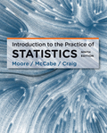
To find: The marginal distribution for the countries of the provided data and the graphical representation of the distribution.
(b)
Answer to Problem 153E
Solution: The obtained marginal totals are shown in the below table.
Country |
Canada |
France |
Germany |
Italy |
Japan |
UK |
US |
Total |
Marginal Percentage |
3.846 |
14.685 |
4.764 |
7.015 |
14.095 |
10.38 |
45.214 |
100 |
And the graphical representation is shown below:

Explanation of Solution
Calculation: To obtain the marginal distribution, below steps are followed in the Minitab software.
Step 1: Enter the data in Minitab worksheet.
Step 2: Go to Stat > Tables > Descriptive Statistics.
Step 3: Select “Field” in “For rows” and select “Country” in “For columns”. And select “Count” in “Frequencies are in”.
Step 4: Select the option “Total percents” and under the “Categorical Variables”.
Step 5: Click OK twice.
The percentage of totals are obtained as the Minitab output. The obtained marginal distribution are shown in the below table.
Country |
Canada |
France |
Germany |
Italy |
Japan |
UK |
US |
Total |
Marginal Percentage |
3.846 |
14.685 |
4.764 |
7.015 |
14.095 |
10.38 |
45.214 |
100 |
Graph: The marginal distribution is graphically shown by using the bar graph. To obtained the graphical representation, below steps are followed in the Minitab software.
Step 1: Insert the data into the worksheet.
Step 2: Go to Graph
Step 3: Click on the drop down menu of “Bar represents” and select “Values from table”.
Step 3: Select “Simple” and click “OK”.
Step 4: Specify the “Graph variables” and “Categorical variable”.
Step 5: Click “OK”.
The bar graph is obtained as:
Interpretation: The maximum percentage of students belongs to US whereas the minimum percentage of the students belongs to Canada.
(c)
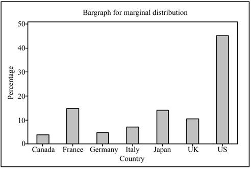
To find: The marginal distribution for the Field of study of the provided data and the graphical representation of the distribution.
(c)
Answer to Problem 153E
Solution: The obtained marginal totals are shown in the below table.
Field of study |
SsBL |
SME |
AH |
Ed |
Other |
Total |
Marginal Percentage |
36.888 |
19.908 |
17.504 |
6.971 |
18.728 |
100 |
And the graphical representation is shown below:
Explanation of Solution
Calculation: To obtained the marginal totals, below steps are followed in the Minitab software.
Step 1: Enter the data in Minitab worksheet.
Step 2: Go to Stat > Tables > Descriptive Statistics.
Step 3: Select “Field” in “For rows” and select “Country” in “For columns”. And select “Count” in “Frequencies are in”.
Step 4: Select the option “Total percents” and under the “Categorical Variables”.
Step 5: Click OK twice.
The percentage of totals are obtained as the Minitab output. The obtained marginal distribution are shown in the below table.
Field of study |
SsBL |
SME |
AH |
Ed |
Other |
Total |
Marginal Percentage |
17.504 |
6.971 |
18.728 |
19.908 |
36.888 |
100 |
Graph: The marginal distribution is graphically shown by using the bar graph. To obtain the graphical representation, below steps are followed in the Minitab software.
Step 1: Insert the data into the worksheet.
Step 2: Go to Graph
Step 3: Click on the drop down menu of “Bar represents” and select “Values from table”.
Step 3: Select “Simple” and click “OK”.
Step 4: Specify the “Graph variables” and “Categorical variable”.
Step 5: Click “OK”.
The bar graph is obtained as:
Interpretation: The maximum percentage of students studies SsBL fields whereas the minimum percentage of the students studies Ed.
Want to see more full solutions like this?
Chapter 2 Solutions
Introduction to the Practice of Statistics


- The details of the clock sales at a supermarket for the past 6 weeks are shown in the table below. The time series appears to be relatively stable, without trend, seasonal, or cyclical effects. The simple moving average value of k is set at 2. If the smoothing constant is assumed to be 0.7, and setting F1 and F2=A1, what is the exponential smoothing sales forecast for week 7? Round to the nearest whole number. Week Units sold 1 88 2 44 3 54 4 65 5 72 6 85 Question content area bottom Part 1 A. 80 clocks B. 60 clocks C. 70 clocks D. 50 clocksarrow_forwardThe details of the clock sales at a supermarket for the past 6 weeks are shown in the table below. The time series appears to be relatively stable, without trend, seasonal, or cyclical effects. The simple moving average value of k is set at 2. Calculate the value of the simple moving average mean absolute percentage error. Round to two decimal places. Week Units sold 1 88 2 44 3 54 4 65 5 72 6 85 Part 1 A. 14.39 B. 25.56 C. 23.45 D. 20.90arrow_forwardThe accompanying data shows the fossil fuels production, fossil fuels consumption, and total energy consumption in quadrillions of BTUs of a certain region for the years 1986 to 2015. Complete parts a and b. Year Fossil Fuels Production Fossil Fuels Consumption Total Energy Consumption1949 28.748 29.002 31.9821950 32.563 31.632 34.6161951 35.792 34.008 36.9741952 34.977 33.800 36.7481953 35.349 34.826 37.6641954 33.764 33.877 36.6391955 37.364 37.410 40.2081956 39.771 38.888 41.7541957 40.133 38.926 41.7871958 37.216 38.717 41.6451959 39.045 40.550 43.4661960 39.869 42.137 45.0861961 40.307 42.758 45.7381962 41.732 44.681 47.8261963 44.037 46.509 49.6441964 45.789 48.543 51.8151965 47.235 50.577 54.0151966 50.035 53.514 57.0141967 52.597 55.127 58.9051968 54.306 58.502 62.4151969 56.286…arrow_forward
- The accompanying data shows the fossil fuels production, fossil fuels consumption, and total energy consumption in quadrillions of BTUs of a certain region for the years 1986 to 2015. Complete parts a and b. Year Fossil Fuels Production Fossil Fuels Consumption Total Energy Consumption1949 28.748 29.002 31.9821950 32.563 31.632 34.6161951 35.792 34.008 36.9741952 34.977 33.800 36.7481953 35.349 34.826 37.6641954 33.764 33.877 36.6391955 37.364 37.410 40.2081956 39.771 38.888 41.7541957 40.133 38.926 41.7871958 37.216 38.717 41.6451959 39.045 40.550 43.4661960 39.869 42.137 45.0861961 40.307 42.758 45.7381962 41.732 44.681 47.8261963 44.037 46.509 49.6441964 45.789 48.543 51.8151965 47.235 50.577 54.0151966 50.035 53.514 57.0141967 52.597 55.127 58.9051968 54.306 58.502 62.4151969 56.286…arrow_forwardThe accompanying data shows the fossil fuels production, fossil fuels consumption, and total energy consumption in quadrillions of BTUs of a certain region for the years 1986 to 2015. Complete parts a and b. Develop line charts for each variable and identify the characteristics of the time series (that is, random, stationary, trend, seasonal, or cyclical). What is the line chart for the variable Fossil Fuels Production?arrow_forwardThe accompanying data shows the fossil fuels production, fossil fuels consumption, and total energy consumption in quadrillions of BTUs of a certain region for the years 1986 to 2015. Complete parts a and b. Year Fossil Fuels Production Fossil Fuels Consumption Total Energy Consumption1949 28.748 29.002 31.9821950 32.563 31.632 34.6161951 35.792 34.008 36.9741952 34.977 33.800 36.7481953 35.349 34.826 37.6641954 33.764 33.877 36.6391955 37.364 37.410 40.2081956 39.771 38.888 41.7541957 40.133 38.926 41.7871958 37.216 38.717 41.6451959 39.045 40.550 43.4661960 39.869 42.137 45.0861961 40.307 42.758 45.7381962 41.732 44.681 47.8261963 44.037 46.509 49.6441964 45.789 48.543 51.8151965 47.235 50.577 54.0151966 50.035 53.514 57.0141967 52.597 55.127 58.9051968 54.306 58.502 62.4151969 56.286…arrow_forward
- For each of the time series, construct a line chart of the data and identify the characteristics of the time series (that is, random, stationary, trend, seasonal, or cyclical). Month PercentApr 1972 4.97May 1972 5.00Jun 1972 5.04Jul 1972 5.25Aug 1972 5.27Sep 1972 5.50Oct 1972 5.73Nov 1972 5.75Dec 1972 5.79Jan 1973 6.00Feb 1973 6.02Mar 1973 6.30Apr 1973 6.61May 1973 7.01Jun 1973 7.49Jul 1973 8.30Aug 1973 9.23Sep 1973 9.86Oct 1973 9.94Nov 1973 9.75Dec 1973 9.75Jan 1974 9.73Feb 1974 9.21Mar 1974 8.85Apr 1974 10.02May 1974 11.25Jun 1974 11.54Jul 1974 11.97Aug 1974 12.00Sep 1974 12.00Oct 1974 11.68Nov 1974 10.83Dec 1974 10.50Jan 1975 10.05Feb 1975 8.96Mar 1975 7.93Apr 1975 7.50May 1975 7.40Jun 1975 7.07Jul 1975 7.15Aug 1975 7.66Sep 1975 7.88Oct 1975 7.96Nov 1975 7.53Dec 1975 7.26Jan 1976 7.00Feb 1976 6.75Mar 1976 6.75Apr 1976 6.75May 1976…arrow_forwardHi, I need to make sure I have drafted a thorough analysis, so please answer the following questions. Based on the data in the attached image, develop a regression model to forecast the average sales of football magazines for each of the seven home games in the upcoming season (Year 10). That is, you should construct a single regression model and use it to estimate the average demand for the seven home games in Year 10. In addition to the variables provided, you may create new variables based on these variables or based on observations of your analysis. Be sure to provide a thorough analysis of your final model (residual diagnostics) and provide assessments of its accuracy. What insights are available based on your regression model?arrow_forwardI want to make sure that I included all possible variables and observations. There is a considerable amount of data in the images below, but not all of it may be useful for your purposes. Are there variables contained in the file that you would exclude from a forecast model to determine football magazine sales in Year 10? If so, why? Are there particular observations of football magazine sales from previous years that you would exclude from your forecasting model? If so, why?arrow_forward
- Stat questionsarrow_forward1) and let Xt is stochastic process with WSS and Rxlt t+t) 1) E (X5) = \ 1 2 Show that E (X5 = X 3 = 2 (= = =) Since X is WSSEL 2 3) find E(X5+ X3)² 4) sind E(X5+X2) J=1 ***arrow_forwardProve that 1) | RxX (T) | << = (R₁ " + R$) 2) find Laplalse trans. of Normal dis: 3) Prove thy t /Rx (z) | < | Rx (0)\ 4) show that evary algebra is algebra or not.arrow_forward
 MATLAB: An Introduction with ApplicationsStatisticsISBN:9781119256830Author:Amos GilatPublisher:John Wiley & Sons Inc
 Probability and Statistics for Engineering and th...StatisticsISBN:9781305251809Author:Jay L. DevorePublisher:Cengage Learning
 Statistics for The Behavioral Sciences (MindTap C...StatisticsISBN:9781305504912Author:Frederick J Gravetter, Larry B. WallnauPublisher:Cengage Learning
 Elementary Statistics: Picturing the World (7th E...StatisticsISBN:9780134683416Author:Ron Larson, Betsy FarberPublisher:PEARSON
 The Basic Practice of StatisticsStatisticsISBN:9781319042578Author:David S. Moore, William I. Notz, Michael A. FlignerPublisher:W. H. Freeman
 Introduction to the Practice of StatisticsStatisticsISBN:9781319013387Author:David S. Moore, George P. McCabe, Bruce A. CraigPublisher:W. H. Freeman