
(a)
The
Answer to Problem 1E
Hence, the price along the vertical axis and the quantity along the horizontal axis has been determined and the first two columns have been plotted.
Explanation of Solution
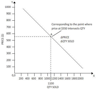
The graph is plotted by joining 3 points of price on Y-axis to the corresponding quantity sold on the X-axis.
To find the quantity sold when the price is a certain dollar, we can take the help of the line obtained by plotting 3 price point in the Y-axis to the corresponding quantity in the x-axis in the graph sheet, and join them to form a sloping straight line.
Once the new quantity is found for a particular price point from the above straight line, we can use this information to find the total revenue at that price.
(b)
The quantity sold when the price is $550.
Answer to Problem 1E
When the price is 550$, the quantity sold is 1100.
Explanation of Solution
From the above-plotted line on the graph, we find that the point when the price on Y-axis is 550$, the corresponding quantity sold on X-axis is 1100 numbers.
To find the quantity sold when the price is a certain dollar, we can take the help of the line obtained by plotting 3 price point in the Y-axis to the corresponding quantity in the x-axis in the graph sheet, and join them to form a sloping straight line.
Once the new quantity is found for a particular price point from the above straight line, we can use this information to find the total revenue at that price.
(c)
To plot a graph and to measure the quantity on the horizontal axis and to determine the total revenue on the vertical axis.
Answer to Problem 1E
The graph is plotted and the quantity sold at 550$ is 1100 numbers.
Explanation of Solution
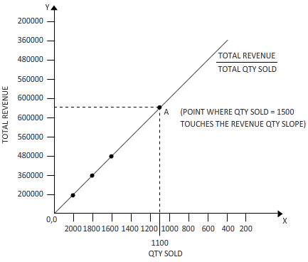
Now in the graph drawn above, the quantity sold is taken on X-axis while the total revenue obtained for that numbers of corresponding quantity sold is taken on Y-AXIS.
Next, we plot the points of total quantity sold on the horizontal X-axis versus the total Revenue obtained by selling each number of that quantity on the vertical Y-Axis. We take such thee points where the quantity-sold and corresponding revenue interacts, and join them to form a straight line.
To find the quantity sold when the price is at a certain dollar, we can take the help of the line obtained by plotting 3 price point in the Y-axis to the corresponding quantity in the x-axis in the graph sheet, and join them to form a sloping straight line.
Once the new quantity is found for a particular price point from the above straight line, we can use this information to find the total revenue at that price.
(d)
The total revenue when the price is $550 and to determine if the total revenue will increase or decrease when the price is lowered.
Answer to Problem 1E
When the quantity sold is $ 550, the total revenue is $ 6,40,000.
Explanation of Solution
We already know the quantity sold at each price point. Conversely, we know the price too when a particular number of items is sold. In this problem, the total revenue is to be found when the price is 550$. Now the corresponding total revenue to 1100 numbers is found to be 6,40,000 on the Y-axis. As we can see from the graph, decrease in price will increase the revenue.
To find the quantity sold when the price is a certain dollar, we can take the help of the line obtained by plotting 3 price point in the Y-axis to the corresponding quantity in the x-axis in the graph sheet, and join them to form a sloping straight line.
Once the new quantity is found for a particular price point from the above straight line, we can use this information to find the total revenue at that price.
Want to see more full solutions like this?
Chapter 1A Solutions
Economics:

- not use ai pleasearrow_forward• Prismatic Cards: A prismatic card will be a card that counts as having every suit. We will denote, e.g., a prismatic Queen card by Q*. With this notation, 2.3045 Q would be a double flush since every card is a diamond and a heart. • Wild Cards: A wild card counts as having every suit and every denomination. Denote wild cards with a W; if there are multiple, we will denote them W₁, W2, etc. With this notation, W2 20.30054 would be both a three-of-a-kind (three 2's) and a flush (5 diamonds). If we add multiple wild cards to the deck, they count as distinct cards, so that (e.g.) the following two hands count as "different hands" when counting: W15 5Q and W255◊♡♡♣♣ In addition, 1. Let's start with the unmodified double-suited deck. (a) Call a hand a flush house if it is a flush and a full house, i.e. if all cards share a suit and there are 3 cards of one denomination and two of another. For example, 550. house. How many different flush house hands are there? 2. Suppose we add one wild…arrow_forwardnot use ai pleasearrow_forward
- In a classic oil-drilling example, you are trying to decide whether to drill for oil on a field that might or might not contain any oil. Before making this decision, you have the option of hiring a geologist to perform some seismic tests and then predict whether there is any oil or not. You assess that if there is actually oil, the geologist will predict there is oil with probability 0.85 . You also assess that if there is no oil, the geologist will predict there is no oil with probability 0.90. Please answer the two questions below, as I am trying to ensure that I am correct. 1. Why will these two probabilities not appear on the decision tree? 2. Which probabilities will be on the decision tree?arrow_forwardAsap pleasearrow_forwardnot use ai pleasearrow_forward
- not use ai pleasearrow_forwardIn this question, you will test relative purchasing parity (PPP) using the data. Use yearly data from FRED website from 1971 to 2020: (i) The Canadian Dollars to U.S. Dollar Spot Exchange Rate (ER) (ii) Consumer price index for Canada (CAN_CPI), and (iii) Consumer price index for the US (US_CPI). Inflation is measured by the consumer price index (CPI). The relative PPP equation is: AE CAN$/US$ ECAN$/US$ = π CAN - πUS Submit the Excel sheet that you worked on. 1. First, compute the percentage change in the exchange rate (left-hand side of the equation). Caculate the variable for each year from 1972 to 2020 in Column E (named Change_ER) of the Excel sheet. For example, for 1972, compute E3: (B3-B2)/B2). ER1972 ER1971 ER 1971 (in Excel, the formula in cellarrow_forwardnot use ai pleasearrow_forward
- 8. The current price of 3M stock is $87 per share. The previous dividend paid was $5.96, and the next dividend is $6.25, assuming a growth rate of 4.86% per year. What is the forward (next 12 months) dividend yield? Show at least two decimal places, as in x.xx% %arrow_forwardJoy's Frozen Yogurt shops have enjoyed rapid growth in northeastern states in recent years. From the analysis of Joy's various outlets, it was found that the demand curve follows this pattern: Q=200-300P+1201 +657-250A +400A; where Q = number of cups served per week P = average price paid for each cup I = per capita income in the given market (thousands) Taverage outdoor temperature A competition's monthly advertising expenditures (thousands) = A; = Joy's own monthly advertising expenditures (thousands) One of the outlets has the following conditions: P = 1.50, I = 10, T = 60, A₁ = 15, A; = 10 1. Estimate the number of cups served per week by this outlet. Also determine the outlet's demand curve. 2. What would be the effect of a $5,000 increase in the competitor's advertising expenditure? Illustrate the effect on the outlet's demand curve. 3. What would Joy's advertising expenditure have to be to counteract this effect?arrow_forwardThe Compute Company store has been selling its special word processing software, Aceword, during the last 10 months. Monthly sales and the price for Aceword are shown in the following table. Also shown are the prices for a competitive software, Goodwrite, and estimates of monthly family income. Calculate the appropriate elasticities, keeping in mind that you can calculate an elasticity measure only when all other factors do not change (using Excel). For example, price elasticities, months 1-2. Month Price Aceword Quantity Aceword Family Income Price Goodwrite 1 $120 200 $4,000 $130 21 120 210 4,000 145 3 120 220 4,200 145 4 110 240 4,200 145 90 5 115 230 4,200 145 6 115 215 4,200 125 10 7899 115 220 4,400 125 105 230 4,400 125 105 235 4,600 125 105 220 4,600 115arrow_forward

 Economics Today and Tomorrow, Student EditionEconomicsISBN:9780078747663Author:McGraw-HillPublisher:Glencoe/McGraw-Hill School Pub Co
 Managerial Economics: Applications, Strategies an...EconomicsISBN:9781305506381Author:James R. McGuigan, R. Charles Moyer, Frederick H.deB. HarrisPublisher:Cengage Learning
 Essentials of Economics (MindTap Course List)EconomicsISBN:9781337091992Author:N. Gregory MankiwPublisher:Cengage Learning
 Exploring EconomicsEconomicsISBN:9781544336329Author:Robert L. SextonPublisher:SAGE Publications, Inc
 Microeconomics: Private and Public Choice (MindTa...EconomicsISBN:9781305506893Author:James D. Gwartney, Richard L. Stroup, Russell S. Sobel, David A. MacphersonPublisher:Cengage Learning