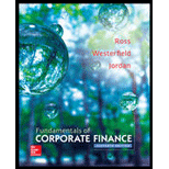
Fundamentals of Corporate Finance
11th Edition
ISBN: 9780077861704
Author: Stephen A. Ross Franco Modigliani Professor of Financial Economics Professor, Randolph W Westerfield Robert R. Dockson Deans Chair in Bus. Admin., Bradford D Jordan Professor
Publisher: McGraw-Hill Education
expand_more
expand_more
format_list_bulleted
Concept explainers
Textbook Question
Chapter 19.A, Problem 8QP
Interpreting Miller–Orr Based on the Miller–Orr model, describe what will happen to the lower limit, the upper limit, and the spread (the distance between the two) if the variation in net cash flow grows. Give an intuitive explanation for why this happens. What happens if the variance drops to zero?
Expert Solution & Answer
Want to see the full answer?
Check out a sample textbook solution
Students have asked these similar questions
Do you know what are Keith Gill's previous projects?
Explain why long-term bonds are subject to greater interest rate risk than short-term bonds with references or practical examples.
What does it mean when a bond is referred to as a convertible bond? Would a convertible bond be more or less attractive to a bond holder than a non-convertible bond? Explain in detail with examples or academic references.
Chapter 19 Solutions
Fundamentals of Corporate Finance
Ch. 19.1 - What is the transaction motive, and how does it...Ch. 19.1 - What is the cost to the firm of holding excess...Ch. 19.2 - Which would a firm be most interested in reducing,...Ch. 19.2 - Prob. 19.2BCQCh. 19.2 - Prob. 19.2CCQCh. 19.3 - Prob. 19.3ACQCh. 19.3 - Prob. 19.3BCQCh. 19.4 - Prob. 19.4ACQCh. 19.4 - What is a zero-balance account? What is the...Ch. 19.5 - What are some reasons why firms find themselves...
Ch. 19.5 - Prob. 19.5BCQCh. 19.5 - Why are money market preferred stocks an...Ch. 19.A - Prob. 1ACQCh. 19.A - Prob. 2BCQCh. 19.A - Describe how the MillerOrr model works.Ch. 19.A - Changes in Target Cash Balances Indicate the...Ch. 19.A - Using the BAT Model Given the following...Ch. 19.A - Prob. 3QPCh. 19.A - Prob. 4QPCh. 19.A - Determining Optimal Cash Balances The All Day...Ch. 19.A - Prob. 6QPCh. 19.A - Prob. 7QPCh. 19.A - Interpreting MillerOrr Based on the MillerOrr...Ch. 19.A - Prob. 9QPCh. 19.A - Using BAT Rise Against Corporation has determined...Ch. 19 - Prob. 19.1CTFCh. 19 - Prob. 19.2CTFCh. 19 - Prob. 19.3CTFCh. 19 - Prob. 1CRCTCh. 19 - Prob. 2CRCTCh. 19 - Prob. 3CRCTCh. 19 - Prob. 4CRCTCh. 19 - Prob. 5CRCTCh. 19 - Prob. 6CRCTCh. 19 - Collection and Disbursement Floats [LO1] Which...Ch. 19 - Prob. 8CRCTCh. 19 - Prob. 9CRCTCh. 19 - Prob. 10CRCTCh. 19 - Prob. 11CRCTCh. 19 - Prob. 12CRCTCh. 19 - Prob. 13CRCTCh. 19 - Prob. 1QPCh. 19 - Calculating Net Float [LO1] Each business day, on...Ch. 19 - Prob. 3QPCh. 19 - Float and Weighted Average Delay [LO1] Your...Ch. 19 - NPV and Collection Time [LO2] Your firm has an...Ch. 19 - Using Weighted Average Delay [LO1] A mail-order...Ch. 19 - Prob. 7QPCh. 19 - Lockboxes and Collections [LO2] It takes Cookie...Ch. 19 - Prob. 9QPCh. 19 - Prob. 10QPCh. 19 - Prob. 11QPCh. 19 - Calculating Transactions Required [LO2] Cow Chips,...Ch. 19 - Prob. 1MCh. 19 - Prob. 2MCh. 19 - Prob. 3M
Knowledge Booster
Learn more about
Need a deep-dive on the concept behind this application? Look no further. Learn more about this topic, finance and related others by exploring similar questions and additional content below.Similar questions
- Alfa international paid $2.00 annual dividend on common stock and promises that the dividend will grow by 4% per year, if the stock’s market price for today is $20, what is required rate of return?arrow_forwardgive answer general accounting.arrow_forwardGive me answers in general financearrow_forward
- General Finance Question Solution Please with calculationarrow_forwardGeneral Financearrow_forwardAs CFO for Everything.Com, you are shopping for 6,000 square feet of usable office space for 25 of your employees in Center City, USA. A leasing broker shows you space in Apex Atrium, a 10-story multitenanted office building. This building contains 360,000 square feet of gross building area. A total of 54,000 square feet is interior space and is nonrentable. The nonrentable space consists of areas contained in the basement, elevator core, and other mechanical and structural components. An additional 36,000 square feet of common area is the lobby area usable by all tenants. The 6,000 square feet of usable area that you are looking for is on the seventh floor, which contains 33,600 square feet of rentable area, and is leased by other tenants who occupy a combined total of 24,000 square feet of usable space. The leasing broker indicated that base rents will be $30 per square foot of rentable area Required: a. Calculate total rentable area in the building as though it would be rented to…arrow_forward
- Don't used Ai solutionarrow_forwardGeneral Finance Questionarrow_forwardConsider the following simplified financial statements for the Yoo Corporation (assuming no income taxes): Income Statement Balance Sheet Sales Costs $ 40,000 Assets 34,160 $26,000 Debt Equity $ 7,000 19,000 Net income $ 5,840 Total $26,000 Total $26,000 The company has predicted a sales increase of 20 percent. Assume Yoo pays out half of net income in the form of a cash dividend. Costs and assets vary with sales, but debt and equity do not. Prepare the pro forma statements. (Input all amounts as positive values. Do not round intermediate calculations and round your answers to the nearest whole dollar amount.) Pro forma income statement Sales Costs $ 48000 40992 Assets $ 31200 Pro forma balance sheet Debt 7000 Equity 19000 Net income $ 7008 Total $ 31200 Total 30304 What is the external financing needed? (Do not round intermediate calculations. Negative amount should be indicated by a minus sign.) External financing needed $ 896arrow_forward
- An insurance company has liabilities of £7 million due in 10 years' time and £9 million due in 17 years' time. The assets of the company consist of two zero-coupon bonds, one paying £X million in 7 years' time and the other paying £Y million in 20 years' time. The current interest rate is 6% per annum effective. Find the nominal value of X (i.e. the amount, IN MILLIONS, that bond X pays in 7 year's time) such that the first two conditions for Redington's theory of immunisation are satisfied. Express your answer to THREE DECIMAL PLACES.arrow_forwardAn individual is investing in a market where spot rates and forward rates apply. In this market, if at time t=0 he agrees to invest £5.3 for two years, he will receive £7.4 at time t=2 years. Alternatively, if at time t=0 he agrees to invest £5.3 at time t=1 for either one year or two years, he will receive £7.5 or £7.3 at times t=2 and t=3, respectively. Calculate the price per £5,000 nominal that the individual should pay for a fixed-interest bond bearing annual interest of 6.6% and is redeemable after 3 years at 110%. State your answer at 2 decimal places.arrow_forwardThe one-year forward rates of interest, f+, are given by: . fo = 5.06%, f₁ = 6.38%, and f2 = 5.73%. Calculate, to 4 decimal places (in percentages), the three-year par yield.arrow_forward
arrow_back_ios
SEE MORE QUESTIONS
arrow_forward_ios
Recommended textbooks for you
 Managerial Accounting: The Cornerstone of Busines...AccountingISBN:9781337115773Author:Maryanne M. Mowen, Don R. Hansen, Dan L. HeitgerPublisher:Cengage Learning
 Essentials of Business Analytics (MindTap Course ...StatisticsISBN:9781305627734Author:Jeffrey D. Camm, James J. Cochran, Michael J. Fry, Jeffrey W. Ohlmann, David R. AndersonPublisher:Cengage Learning
 EBK CONTEMPORARY FINANCIAL MANAGEMENTFinanceISBN:9781337514835Author:MOYERPublisher:CENGAGE LEARNING - CONSIGNMENT
 Intermediate Financial Management (MindTap Course...FinanceISBN:9781337395083Author:Eugene F. Brigham, Phillip R. DavesPublisher:Cengage Learning

Managerial Accounting: The Cornerstone of Busines...
Accounting
ISBN:9781337115773
Author:Maryanne M. Mowen, Don R. Hansen, Dan L. Heitger
Publisher:Cengage Learning

Essentials of Business Analytics (MindTap Course ...
Statistics
ISBN:9781305627734
Author:Jeffrey D. Camm, James J. Cochran, Michael J. Fry, Jeffrey W. Ohlmann, David R. Anderson
Publisher:Cengage Learning

EBK CONTEMPORARY FINANCIAL MANAGEMENT
Finance
ISBN:9781337514835
Author:MOYER
Publisher:CENGAGE LEARNING - CONSIGNMENT

Intermediate Financial Management (MindTap Course...
Finance
ISBN:9781337395083
Author:Eugene F. Brigham, Phillip R. Daves
Publisher:Cengage Learning
Portfolio Management; Author: DevTechFinance;https://www.youtube.com/watch?v=Qmw15cG2Mv4;License: Standard YouTube License, CC-BY