Chapter 18, Problem 16P

To determine

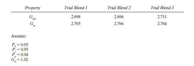
The initial trial asphalt content for different blends.

Answer to Problem 16P

  $4.65\%,$

  $4.69\%$

  $\text{and}44.45\%$

Explanation of Solution

Given information:

Nominal maximum sieve of each aggregate blend = 19 mm.

  

Calculation:

For trial blend 1, we have:

The amount of asphalt binder absorbed by the aggregates is estimated

from Eq. 18.18 as

  $V_{ba}=\frac{P_s\left(1-V_a\right)}{\frac{P_b}{G_b}+\frac{P_s}{G_{se}}}\left[\frac{1}{G_{sb}}-\frac{1}{G_{se}}\right]$

Where, $V_{ba}$ is the volume of absorbed binder, cm3/cm3 of mix,

  $P_b$ is the percent of binder (assumed $0.05$ ),

  $P_s$ is the percent of aggregate (assumed $0.95$ ),

  $G_b$ is the specific gravity of binder (assumed $1.02$ ),

  $G_{se}$ is the effective specific gravity of the aggregate blend

  $G_{sb}$ is the bulk specific gravity of the aggregate blend

  $V_a$ is thevolume of air voids (assumed $0.04cm3/cm3ofmix$ ).

Substitute the values in the required equation, we have

  $\begin{array}{l}{V}_{ba}=\frac{P_s\left(1-V_a\right)}{\frac{P_b}{G_b}+\frac{P_s}{G_{se}}}\left[\frac{1}{G_{sb}}-\frac{1}{G_{se}}\right]\\ V_{ba}=\frac{0.95\left(1-0.04\right)}{\frac{0.05}{1.02}+\frac{0.95}{2.765}}\left[\frac{1}{2.698}-\frac{1}{2.765}\right]\\ V_{ba}=\frac{0.95\left(0.96\right)}{0.049+0.3436}\left[0.371-0.362\right]\\ V_{ba}=\frac{0.912}{0.3926}\left[0.009\right]\\ V_{ba}=\mathrm{0.0209.}\end{array}$

Estimate the percent of effective asphalt binder by volume using theempirical expression given as follows:

  $V_{be}=0.176-(0.0675)\log S_n$

Where, $V_{be}$ is the volume of effective binder content,

  $S_n$ is the nominal maximum sieve size of the total aggregate in the trial aggregate

gradation (mm).

Substitute the values in the required equation, we have

  $\begin{array}{l}{V}_{be}=0.176-(0.0675)\log (19)\\ V_{be}=0.176-(0.0675)\left(1.2788\right)\\ V_{be}=0.176-0.0863.\\ V_{be}=0.0896.\end{array}$

Now, calculate the mass of aggregate by using the following formula:

  $W_S=\frac{P_s\left(1-V_a\right)}{\frac{P_b}{G_b}+\frac{P_s}{G_{se}}}$

Where, $W_S$ is the mass of aggregate

Substitute the values, we have

  $\begin{array}{l}{W}_S=\frac{0.95\left(1-0.04\right)}{\frac{0.05}{1.02}+\frac{0.95}{2.765}}\\ W_S=\frac{0.95\left(0.96\right)}{0.049+0.3436}\\ W_S=\frac{0.912}{0.3926}\\ W_S=2.323grams.\end{array}$

A trial percentage of asphalt binder then is determined for each trial

aggregate blend using the following equation.

  $P_{bi}=\frac{G_b\left(V_{be}+V_{ba}\right)}{\left(G_b\left(V_{be}+V_{ba}\right)\right)+W_s}\times 100$ where

Where, $P_{bi}$ is the percent of binder by mass of mix.

Substitute the values, we have

  $\begin{array}{l}{P}_{bi}=\frac{1.02\left(0.090+0.021\right)}{\left(1.02\left(0.090+0.021\right)\right)+2.323}\times 100\\ P_{bi}=\frac{1.02\left(0.111\right)}{\left(1.02\left(0.111\right)\right)+2.323}\times 100\\ P_{bi}=\frac{0.11322}{0.11322+2.323}\times 100\\ P_{bi}=\frac{11.322}{2.43622}\\ P_{bi}=4.647\\ P_{bi}=4.65\%.\end{array}$

For trial blend 2, we have:

The amount of asphalt binder absorbed by the aggregates is estimated

from Eq. 18.18 as

  $V_{ba}=\frac{P_s\left(1-V_a\right)}{\frac{P_b}{G_b}+\frac{P_s}{G_{se}}}\left[\frac{1}{G_{sb}}-\frac{1}{G_{se}}\right]$

Where, $V_{ba}$ is the volume of absorbed binder, cm3/cm3 of mix,

  $P_b$ is the percent of binder (assumed $0.05$ ),

  $P_s$ is the percent of aggregate (assumed $0.95$ ),

  $G_b$ is the specific gravity of binder (assumed $1.02$ ),

  $G_{se}$ is the effective specific gravity of the aggregate blend

  $G_{sb}$ is the bulk specific gravity of the aggregate blend

  $V_a$ is the volume of air voids (assumed $0.04cm3/cm3ofmix$ ).

Substitute the values in the required equation, we have

  $\begin{array}{l}{V}_{ba}=\frac{P_s\left(1-V_a\right)}{\frac{P_b}{G_b}+\frac{P_s}{G_{se}}}\left[\frac{1}{G_{sb}}-\frac{1}{G_{se}}\right]\\ V_{ba}=\frac{0.95\left(1-0.04\right)}{\frac{0.05}{1.02}+\frac{0.95}{2.766}}\left[\frac{1}{2.698}-\frac{1}{2.766}\right]\\ V_{ba}=\frac{0.95\left(0.96\right)}{0.049+0.3434}\left[0.371-0.361\right]\\ V_{ba}=\frac{0.912}{0.3924}\left[0.01\right]\\ V_{ba}=\mathrm{0.023.}\end{array}$

Estimate the percent of effective asphalt binder by volume using the empirical expression given as follows:

  $V_{be}=0.176-(0.0675)\log S_n$

Where, $V_{be}$ is the volume of effective binder content,

  $S_n$ is the nominal maximum sieve size of the total aggregate in the trial aggregate

gradation (mm).

Substitute the values in the required equation, we have

  $\begin{array}{l}{V}_{be}=0.176-(0.0675)\log (19)\\ V_{be}=0.176-(0.0675)\left(1.2788\right)\\ V_{be}=0.176-0.0863.\\ V_{be}=0.0896.\end{array}$

Now, calculate the mass of aggregate by using the following formula:

  $W_S=\frac{P_s\left(1-V_a\right)}{\frac{P_b}{G_b}+\frac{P_s}{G_{se}}}$

Where, $W_S$ is the mass of aggregate

Substitute the values, we have

  $\begin{array}{l}{W}_S=\frac{0.95\left(1-0.04\right)}{\frac{0.05}{1.02}+\frac{0.95}{2.766}}\\ W_S=\frac{0.95\left(0.96\right)}{0.049+0.3434}\\ W_S=\frac{0.912}{0.3924}\\ W_S=2.324grams.\end{array}$

A trial percentage of asphalt binder then is determined for each trial

aggregate blend using the following equation.

  $P_{bi}=\frac{G_b\left(V_{be}+V_{ba}\right)}{\left(G_b\left(V_{be}+V_{ba}\right)\right)+W_s}\times 100$ where

Where, $P_{bi}$ is the percent of binder by mass of mix.

Substitute the values, we have

  $\begin{array}{l}{P}_{bi}=\frac{1.02\left(0.090+0.022\right)}{\left(1.02\left(0.090+0.022\right)\right)+2.324}\times 100\\ P_{bi}=\frac{1.02\left(0.112\right)}{\left(1.02\left(0.112\right)\right)+2.324}\times 100\\ P_{bi}=\frac{0.11424}{0.11424+2.324}\times 100\\ P_{bi}=\frac{11.424}{2.43824}\\ P_{bi}=4.685\\ P_{bi}=4.69\%.\end{array}$

For trial blend 3, we have:

The amount of asphalt binder absorbed by the aggregates is estimated

from Eq. 18.18 as

  $V_{ba}=\frac{P_s\left(1-V_a\right)}{\frac{P_b}{G_b}+\frac{P_s}{G_{se}}}\left[\frac{1}{G_{sb}}-\frac{1}{G_{se}}\right]$

Where, $V_{ba}$ is the volume of absorbed binder, cm3/cm3 of mix,

  $P_b$ is the percent of binder (assumed $0.05$ ),

  $P_s$ is the percent of aggregate (assumed $0.95$ ),

  $G_b$ is the specific gravity of binder (assumed $1.02$ ),

  $G_{se}$ is the effective specific gravity of the aggregate blend

  $G_{sb}$ is the bulk specific gravity of the aggregate blend

  $V_a$ is the volume of air voids (assumed $0.04cm3/cm3ofmix$ ).

Substitute the values in the required equation, we have

  $\begin{array}{l}{V}_{ba}=\frac{P_s\left(1-V_a\right)}{\frac{P_b}{G_b}+\frac{P_s}{G_{se}}}\left[\frac{1}{G_{sb}}-\frac{1}{G_{se}}\right]\\ V_{ba}=\frac{0.95\left(1-0.04\right)}{\frac{0.05}{1.02}+\frac{0.95}{2.764}}\left[\frac{1}{2.711}-\frac{1}{2.764}\right]\\ V_{ba}=\frac{0.95\left(0.96\right)}{0.0490+0.3437}\left[0.3688-0.3618\right]\\ V_{ba}=\frac{0.912}{0.3927}\left[0.0070\right]\\ V_{ba}=\mathrm{0.01626.}\\ V_{ba}=0.0163.\end{array}$

Estimate the percent of effective asphalt binder by volume using the empirical expression given as follows:

  $V_{be}=0.176-(0.0675)\log S_n$

Where, $V_{be}$ is the volume of effective binder content,

  $S_n$ is the nominal maximum sieve size of the total aggregate in the trial aggregate

gradation (mm).

Substitute the values in the required equation, we have

  $\begin{array}{l}{V}_{be}=0.176-(0.0675)\log (19)\\ V_{be}=0.176-(0.0675)\left(1.2788\right)\\ V_{be}=0.176-0.0863.\\ V_{be}=0.0896.\end{array}$

Now, calculate the mass of aggregate by using the following formula:

  $W_S=\frac{P_s\left(1-V_a\right)}{\frac{P_b}{G_b}+\frac{P_s}{G_{se}}}$

Where, $W_S$ is the mass of aggregate

Substitute the values, we have

  $\begin{array}{l}{W}_S=\frac{0.95\left(1-0.04\right)}{\frac{0.05}{1.02}+\frac{0.95}{2.764}}\\ W_S=\frac{0.95\left(0.96\right)}{0.049+0.3437}\\ W_S=\frac{0.912}{0.3927}\\ W_S=2.322grams.\end{array}$

A trial percentage of asphalt binder then is determined for each trial

aggregate blend using the following equation.

  $P_{bi}=\frac{G_b\left(V_{be}+V_{ba}\right)}{\left(G_b\left(V_{be}+V_{ba}\right)\right)+W_s}\times 100$ where

Where, $P_{bi}$ is the percent of binder by mass of mix.

Substitute the values, we have

  $\begin{array}{l}{P}_{bi}=\frac{1.02\left(0.090+0.016\right)}{\left(1.02\left(0.090+0.016\right)\right)+2.322}\times 100\\ P_{bi}=\frac{1.02\left(0.106\right)}{\left(1.02\left(0.106\right)\right)+2.322}\times 100\\ P_{bi}=\frac{0.10812}{0.10812+2.324}\times 100\\ P_{bi}=\frac{108.12}{2.43212}\\ P_{bi}=44.45\%.\end{array}$

Conclusion:

Therefore, the initial trial asphalt content for1^st, 2^nd and 3^rd blends is as follows $4.65\%,$ $4.69\%$ and $44.45\%$ respectively.