Concept explainers
Videos
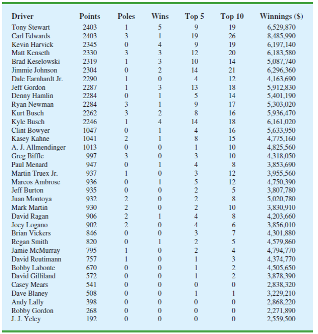
Matt Kenseth won the 2012 Daytona 500, the most important race of the NASCAR season. His win was no surprise because for the 2011 season he finished fourth in the point standings with 2330 points, behind Tony Stewart (2403 points), Carl Edwards (2403 points), and Kevin Harvick (2345 points). In 2011 he earned $6,183,580 by winning three Poles (fastest driver in qualifying), winning three races, finishing in the top five 12 times, and finishing in the top ten 20 times. NASCAR’s point system in 2011 allocated 43 points to the driver who finished first, 42 points to the driver who finished second, and so on down to 1 point for the driver who finished in the 43rd position. In addition any driver who led a lap received 1 bonus point, the driver who led the most laps received an additional bonus point, and the race winner was awarded 3 bonus points. But, the maximum number of points a driver could earn in any race was 48. Table 15.13 shows data for the 2011 season for the top 35 drivers (NASCAR website, February 28, 2011).
TABLE 15.13 NASCAR RESULTS FOR THE 2011 SEASON
Managerial Report
- 1. Suppose you wanted to predict Winnings ($) using only the number of poles won (Poles), the number of wins (Wins), the number of top five finishes (Top 5), or the number of top ten finishes (Top 10). Which of these four variables provides the best single predictor of winnings?
- 2. Develop an estimated regression equation that can be used to predict Winnings ($) given the number of poles won (Poles), the number of wins (Wins), the number of top five finishes (Top 5), and the number of top ten (Top 10) finishes. Test for individual significance and discuss your findings and conclusions.
- 3. Create two new independent variables: Top 2-5 and Top 6-10. Top 2-5 represents the number of times the driver finished between second and fifth place and Top 6-10 represents the number of times the driver finished between sixth and tenth place. Develop an estimated regression equation that can be used to predict Winnings ($) using Poles, Wins, Top 2-5, and Top 6-10. Test for individual significance and discuss your findings and conclusions.
- 4. Based upon the results of your analysis, what estimated regression equation would you recommend using to predict Winnings ($)? Provide an interpretation of the estimated regression coefficients for this equation.

Trending nowThis is a popular solution!

Chapter 15 Solutions
STATISTICS F/BUSINESS+ECONOMICS-TEXT


- What were the average sales for the four weeks prior to the experiment? What were the sales during the four weeks when the stores used the digital display? What is the mean difference in sales between the experimental and regular POP time periods? State the null hypothesis being tested by the paired sample t-test. Do you reject or retain the null hypothesis? At a 95% significance level, was the difference significant? Explain why or why not using the results from the paired sample t-test. Should the manager of the retail chain install new digital displays in each store? Justify your answer.arrow_forwardA retail chain is interested in determining whether a digital video point-of-purchase (POP) display would stimulate higher sales for a brand advertised compared to the standard cardboard point-of-purchase display. To test this, a one-shot static group design experiment was conducted over a four-week period in 100 different stores. Fifty stores were randomly assigned to the control treatment (standard display) and the other 50 stores were randomly assigned to the experimental treatment (digital display). Compare the sales of the control group (standard POP) to the experimental group (digital POP). What were the average sales for the standard POP display (control group)? What were the sales for the digital display (experimental group)? What is the (mean) difference in sales between the experimental group and control group? List the null hypothesis being tested. Do you reject or retain the null hypothesis based on the results of the independent t-test? Was the difference between the…arrow_forwardQuestion 4 An article in Quality Progress (May 2011, pp. 42-48) describes the use of factorial experiments to improve a silver powder production process. This product is used in conductive pastes to manufacture a wide variety of products ranging from silicon wafers to elastic membrane switches. Powder density (g/cm²) and surface area (cm/g) are the two critical characteristics of this product. The experiments involved three factors: reaction temperature, ammonium percentage, stirring rate. Each of these factors had two levels, and the design was replicated twice. The design is shown in Table 3. A222222222222233 Stir Rate (RPM) Ammonium (%) Table 3: Silver Powder Experiment from Exercise 13.23 Temperature (°C) Density Surface Area 100 8 14.68 0.40 100 8 15.18 0.43 30 100 8 15.12 0.42 30 100 17.48 0.41 150 7.54 0.69 150 8 6.66 0.67 30 150 8 12.46 0.52 30 150 8 12.62 0.36 100 40 10.95 0.58 100 40 17.68 0.43 30 100 40 12.65 0.57 30 100 40 15.96 0.54 150 40 8.03 0.68 150 40 8.84 0.75 30 150…arrow_forward
- - + ++ Table 2: Crack Experiment for Exercise 2 A B C D Treatment Combination (1) Replicate I II 7.037 6.376 14.707 15.219 |++++ 1 བྱ॰༤༠སྦྱོ སྦྱོཋཏྟཱུ a b ab 11.635 12.089 17.273 17.815 с ас 10.403 10.151 4.368 4.098 bc abc 9.360 9.253 13.440 12.923 d 8.561 8.951 ad 16.867 17.052 bd 13.876 13.658 abd 19.824 19.639 cd 11.846 12.337 acd 6.125 5.904 bcd 11.190 10.935 abcd 15.653 15.053 Question 3 Continuation of Exercise 2. One of the variables in the experiment described in Exercise 2, heat treatment method (C), is a categorical variable. Assume that the remaining factors are continuous. (a) Write two regression models for predicting crack length, one for each level of the heat treatment method variable. What differences, if any, do you notice in these two equations? (b) Generate appropriate response surface contour plots for the two regression models in part (a). (c) What set of conditions would you recommend for the factors A, B, and D if you use heat treatment method C = +? (d) Repeat…arrow_forwardQuestion 2 A nickel-titanium alloy is used to make components for jet turbine aircraft engines. Cracking is a potentially serious problem in the final part because it can lead to nonrecoverable failure. A test is run at the parts producer to determine the effect of four factors on cracks. The four factors are: pouring temperature (A), titanium content (B), heat treatment method (C), amount of grain refiner used (D). Two replicates of a 24 design are run, and the length of crack (in mm x10-2) induced in a sample coupon subjected to a standard test is measured. The data are shown in Table 2. 1 (a) Estimate the factor effects. Which factor effects appear to be large? (b) Conduct an analysis of variance. Do any of the factors affect cracking? Use a = 0.05. (c) Write down a regression model that can be used to predict crack length as a function of the significant main effects and interactions you have identified in part (b). (d) Analyze the residuals from this experiment. (e) Is there an…arrow_forwardA 24-1 design has been used to investigate the effect of four factors on the resistivity of a silicon wafer. The data from this experiment are shown in Table 4. Table 4: Resistivity Experiment for Exercise 5 Run A B с D Resistivity 1 23 2 3 4 5 6 7 8 9 10 11 12 I+I+I+I+Oooo 0 0 ||++TI++o000 33.2 4.6 31.2 9.6 40.6 162.4 39.4 158.6 63.4 62.6 58.7 0 0 60.9 3 (a) Estimate the factor effects. Plot the effect estimates on a normal probability scale. (b) Identify a tentative model for this process. Fit the model and test for curvature. (c) Plot the residuals from the model in part (b) versus the predicted resistivity. Is there any indication on this plot of model inadequacy? (d) Construct a normal probability plot of the residuals. Is there any reason to doubt the validity of the normality assumption?arrow_forward
- Stem1: 1,4 Stem 2: 2,4,8 Stem3: 2,4 Stem4: 0,1,6,8 Stem5: 0,1,2,3,9 Stem 6: 2,2 What’s the Min,Q1, Med,Q3,Max?arrow_forwardAre the t-statistics here greater than 1.96? What do you conclude? colgPA= 1.39+0.412 hsGPA (.33) (0.094) Find the P valuearrow_forwardA poll before the elections showed that in a given sample 79% of people vote for candidate C. How many people should be interviewed so that the pollsters can be 99% sure that from 75% to 83% of the population will vote for candidate C? Round your answer to the whole number.arrow_forward
- Suppose a random sample of 459 married couples found that 307 had two or more personality preferences in common. In another random sample of 471 married couples, it was found that only 31 had no preferences in common. Let p1 be the population proportion of all married couples who have two or more personality preferences in common. Let p2 be the population proportion of all married couples who have no personality preferences in common. Find a95% confidence interval for . Round your answer to three decimal places.arrow_forwardA history teacher interviewed a random sample of 80 students about their preferences in learning activities outside of school and whether they are considering watching a historical movie at the cinema. 69 answered that they would like to go to the cinema. Let p represent the proportion of students who want to watch a historical movie. Determine the maximal margin of error. Use α = 0.05. Round your answer to three decimal places. arrow_forwardA random sample of medical files is used to estimate the proportion p of all people who have blood type B. If you have no preliminary estimate for p, how many medical files should you include in a random sample in order to be 99% sure that the point estimate will be within a distance of 0.07 from p? Round your answer to the next higher whole number.arrow_forward
 Algebra: Structure And Method, Book 1AlgebraISBN:9780395977224Author:Richard G. Brown, Mary P. Dolciani, Robert H. Sorgenfrey, William L. ColePublisher:McDougal Littell
 Algebra for College StudentsAlgebraISBN:9781285195780Author:Jerome E. Kaufmann, Karen L. SchwittersPublisher:Cengage Learning
 Intermediate AlgebraAlgebraISBN:9781285195728Author:Jerome E. Kaufmann, Karen L. SchwittersPublisher:Cengage Learning