Concept explainers
Videos
Matt Kenseth won the 2012 Daytona 500, the most important race of the NASCAR season. His win was no surprise because for the 2011 season he finished fourth in the point standings with 2330 points, behind Tony Stewart (2403 points), Carl Edwards (2403 points), and Kevin Harvick (2345 points). In 2011 he earned $6,183,580 by winning three Poles (fastest driver in qualifying), winning three races, finishing in the top five 12 times, and finishing in the top ten 20 times. NASCAR’s point system in 2011 allocated 43 points to the driver who finished first, 42 points to the driver who finished second, and so on down to 1 point for the driver who finished in the 43rd position. In addition any driver who led a lap received 1 bonus point, the driver who led the most laps received an additional bonus point, and the race winner was awarded 3 bonus points. But, the maximum number of points a driver could earn in any race was 48. Table 15.13 shows data for the 2011 season for the top 35 drivers (NASCAR website).
Managerial Report
- 1. Suppose you wanted to predict Winnings ($) using only the number of poles won (Poles), the number of wins (Wins), the number of top five finishes (Top 5), or the number of top ten finishes (Top 10). Which of these four variables provides the best single predictor of winnings?
- 2. Develop an estimated regression equation that can be used to predict Winnings ($) given the number of poles won (Poles), the number of wins (Wins), the number of top five finishes (Top 5), and the number of top ten (Top 10) finishes. Test for individual significance and discuss your findings and conclusions.
- 3. Create two new independent variables: Top 2–5 and Top 6–10. Top 2–5 represents the number of times the driver finished between second and fifth place and Top 6–10 represents the number of times the driver finished between sixth and tenth place. Develop an estimated regression equation that can be used to predict Winnings ($) using Poles, Wins, Top 2–5, and Top 6–10. Test for individual significance and discuss your findings and conclusions.
TABLE 15.13 Nascar Results for the 2011 Season
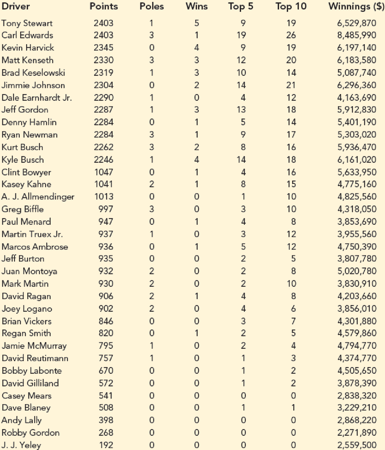
Source: NASCAR website, February 28, 2011. (https://www.nascar.com/)
- 4. Based upon the results of your analysis, what estimated regression equation would you recommend using to predict Winnings ($)? Provide an interpretation of the estimated regression coefficients for this equation.

Trending nowThis is a popular solution!

Chapter 15 Solutions
Essentials of Statistics for Business and Economics (with XLSTAT Printed Access Card)


- According to an economist from a financial company, the average expenditures on "furniture and household appliances" have been lower for households in the Montreal area than those in the Quebec region. A random sample of 14 households from the Montreal region and 16 households from the Quebec region was taken, providing the following data regarding expenditures in this economic sector. It is assumed that the data from each population are distributed normally. We are interested in knowing if the variances of the populations are equal. a) Perform the appropriate hypothesis test on two variances at a significance level of 1%. Include the following information: i. Hypothesis / Identification of populations ii. Critical F-value(s) iii. Decision rule iv. F-ratio value v. Decision and conclusion b) Based on the results obtained in a), is the hypothesis of equal variances for this socio-economic characteristic measured in these two populations upheld? c) Based on the results obtained in a),…arrow_forwardA major company in the Montreal area, offering a range of engineering services from project preparation to construction execution, and industrial project management, wants to ensure that the individuals who are responsible for project cost estimation and bid preparation demonstrate a certain uniformity in their estimates. The head of civil engineering and municipal services decided to structure an experimental plan to detect if there could be significant differences in project evaluation. Seven projects were selected, each of which had to be evaluated by each of the two estimators, with the order of the projects submitted being random. The obtained estimates are presented in the table below. a) Complete the table above by calculating: i. The differences (A-B) ii. The sum of the differences iii. The mean of the differences iv. The standard deviation of the differences b) What is the value of the t-statistic? c) What is the critical t-value for this test at a significance level of 1%?…arrow_forwardCompute the relative risk of falling for the two groups (did not stop walking vs. did stop). State/interpret your result verbally.arrow_forward
- Microsoft Excel include formulasarrow_forwardQuestion 1 The data shown in Table 1 are and R values for 24 samples of size n = 5 taken from a process producing bearings. The measurements are made on the inside diameter of the bearing, with only the last three decimals recorded (i.e., 34.5 should be 0.50345). Table 1: Bearing Diameter Data Sample Number I R Sample Number I R 1 34.5 3 13 35.4 8 2 34.2 4 14 34.0 6 3 31.6 4 15 37.1 5 4 31.5 4 16 34.9 7 5 35.0 5 17 33.5 4 6 34.1 6 18 31.7 3 7 32.6 4 19 34.0 8 8 33.8 3 20 35.1 9 34.8 7 21 33.7 2 10 33.6 8 22 32.8 1 11 31.9 3 23 33.5 3 12 38.6 9 24 34.2 2 (a) Set up and R charts on this process. Does the process seem to be in statistical control? If necessary, revise the trial control limits. [15 pts] (b) If specifications on this diameter are 0.5030±0.0010, find the percentage of nonconforming bearings pro- duced by this process. Assume that diameter is normally distributed. [10 pts] 1arrow_forward4. (5 pts) Conduct a chi-square contingency test (test of independence) to assess whether there is an association between the behavior of the elderly person (did not stop to talk, did stop to talk) and their likelihood of falling. Below, please state your null and alternative hypotheses, calculate your expected values and write them in the table, compute the test statistic, test the null by comparing your test statistic to the critical value in Table A (p. 713-714) of your textbook and/or estimating the P-value, and provide your conclusions in written form. Make sure to show your work. Did not stop walking to talk Stopped walking to talk Suffered a fall 12 11 Totals 23 Did not suffer a fall | 2 Totals 35 37 14 46 60 Tarrow_forward
- Question 2 Parts manufactured by an injection molding process are subjected to a compressive strength test. Twenty samples of five parts each are collected, and the compressive strengths (in psi) are shown in Table 2. Table 2: Strength Data for Question 2 Sample Number x1 x2 23 x4 x5 R 1 83.0 2 88.6 78.3 78.8 3 85.7 75.8 84.3 81.2 78.7 75.7 77.0 71.0 84.2 81.0 79.1 7.3 80.2 17.6 75.2 80.4 10.4 4 80.8 74.4 82.5 74.1 75.7 77.5 8.4 5 83.4 78.4 82.6 78.2 78.9 80.3 5.2 File Preview 6 75.3 79.9 87.3 89.7 81.8 82.8 14.5 7 74.5 78.0 80.8 73.4 79.7 77.3 7.4 8 79.2 84.4 81.5 86.0 74.5 81.1 11.4 9 80.5 86.2 76.2 64.1 80.2 81.4 9.9 10 75.7 75.2 71.1 82.1 74.3 75.7 10.9 11 80.0 81.5 78.4 73.8 78.1 78.4 7.7 12 80.6 81.8 79.3 73.8 81.7 79.4 8.0 13 82.7 81.3 79.1 82.0 79.5 80.9 3.6 14 79.2 74.9 78.6 77.7 75.3 77.1 4.3 15 85.5 82.1 82.8 73.4 71.7 79.1 13.8 16 78.8 79.6 80.2 79.1 80.8 79.7 2.0 17 82.1 78.2 18 84.5 76.9 75.5 83.5 81.2 19 79.0 77.8 20 84.5 73.1 78.2 82.1 79.2 81.1 7.6 81.2 84.4 81.6 80.8…arrow_forwardName: Lab Time: Quiz 7 & 8 (Take Home) - due Wednesday, Feb. 26 Contingency Analysis (Ch. 9) In lab 5, part 3, you will create a mosaic plot and conducted a chi-square contingency test to evaluate whether elderly patients who did not stop walking to talk (vs. those who did stop) were more likely to suffer a fall in the next six months. I have tabulated the data below. Answer the questions below. Please show your calculations on this or a separate sheet. Did not stop walking to talk Stopped walking to talk Totals Suffered a fall Did not suffer a fall Totals 12 11 23 2 35 37 14 14 46 60 Quiz 7: 1. (2 pts) Compute the odds of falling for each group. Compute the odds ratio for those who did not stop walking vs. those who did stop walking. Interpret your result verbally.arrow_forwardSolve please and thank you!arrow_forward
- 7. In a 2011 article, M. Radelet and G. Pierce reported a logistic prediction equation for the death penalty verdicts in North Carolina. Let Y denote whether a subject convicted of murder received the death penalty (1=yes), for the defendant's race h (h1, black; h = 2, white), victim's race i (i = 1, black; i = 2, white), and number of additional factors j (j = 0, 1, 2). For the model logit[P(Y = 1)] = a + ß₁₂ + By + B²², they reported = -5.26, D â BD = 0, BD = 0.17, BY = 0, BY = 0.91, B = 0, B = 2.02, B = 3.98. (a) Estimate the probability of receiving the death penalty for the group most likely to receive it. [4 pts] (b) If, instead, parameters used constraints 3D = BY = 35 = 0, report the esti- mates. [3 pts] h (c) If, instead, parameters used constraints Σ₁ = Σ₁ BY = Σ; B = 0, report the estimates. [3 pts] Hint the probabilities, odds and odds ratios do not change with constraints.arrow_forwardSolve please and thank you!arrow_forwardSolve please and thank you!arrow_forward
 Algebra: Structure And Method, Book 1AlgebraISBN:9780395977224Author:Richard G. Brown, Mary P. Dolciani, Robert H. Sorgenfrey, William L. ColePublisher:McDougal Littell
 Algebra for College StudentsAlgebraISBN:9781285195780Author:Jerome E. Kaufmann, Karen L. SchwittersPublisher:Cengage Learning
 Intermediate AlgebraAlgebraISBN:9781285195728Author:Jerome E. Kaufmann, Karen L. SchwittersPublisher:Cengage Learning