
Videos
State the null and alternative hypothesis.
Find the degrees of freedom for the
Find the critical value of chi-square from Appendix E or from Excel’s
Calculate the chi-square test statistics at 0.10 level of significance and interpret the p-value.
Check whether the conclusion is sensitive to the level of significance chosen, identify the cells that contribute to the chi-square test statistic and check for the small expected frequencies.
Calculate the p-value using Excel’s function if necessary.
Perform a two-tailed, two-sample z test for
Answer to Problem 21CE
The null hypothesis is:
And the alternative hypothesis is:
The degrees of freedom for the contingency table is 1.
The critical-value using EXCEL is 2.706.
There is no enough evidence to conclude that grade and order handed in are independent.
The p-value for the hypothesis test is 0.382.
The conclusion is not sensitive to the level of significance chosen.
The cells (1, 1) and (1, 2) contribute the most to the chi-square test statistic.
There is no expected frequencies that are too small.
It is verified that
Explanation of Solution
Calculation:
The table summarizes the grade and order of papers handed in.
The claim is to test whether the data provide sufficient evidence to conclude that the grade and order handed in are independent. If the claim is rejected, then the grade and order handed in are not independent.
The test hypotheses are given below:
Null hypothesis:
Alternative hypothesis:
The degrees of freedom can be obtained as follows:
Substitute 2 for r and 2 for c.
Thus, the degrees of freedom for the contingency table is 1.
Procedure for critical-value using EXCEL:
Step-by-step software procedure to obtain critical-value using EXCEL software is as follows:
- Open an EXCEL file.
- In cell A1, enter the formula “=CHISQ.INV.RT(0.10,1)”
- Output using EXCEL software is given below:

Thus, the critical-value using EXCEL is 2.706.
Test statistic:
Software procedure:
Step by step procedure to obtain the chi-square test statistics and p-value using the MINITAB software:
- Choose Stat > Tables >Cross Tabulation and Chi-Square.
- Choose Row data (categorical variables).
- In Rows, choose Grade.
- In Columns, choose Order handed in.
- In Frequencies, choose Count.
- In Display, select Counts.
- In chi-square, select Chi-square test, Expected cell counts and Each cell’s contribution to chi-square.
- Click OK.
Output using the MINITAB software is given below:
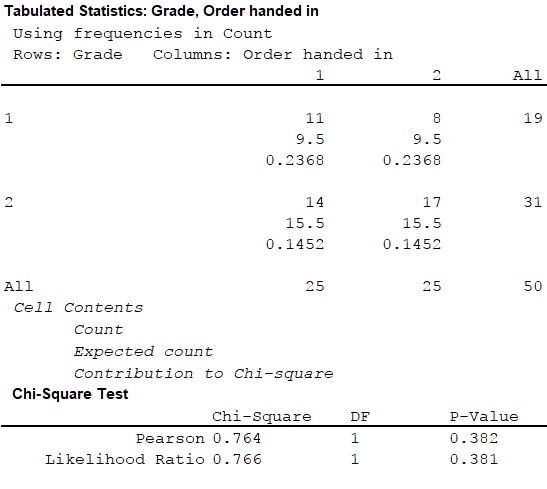
Thus, the test statistic is 0.764 and the p-value for the hypothesis test is 0.382.
Rejection rule:
If the p-value is less than or equal to the significance level, then reject the null hypothesis
Conclusion:
Here, the p-value is greater than the level of significance.
That is,
Therefore, the null hypothesis is not rejected.
Thus, the data provide sufficient evidence to conclude that the grade and order handed in are independent.
Take
Here, the p-value is greater than the level of significance.
That is,
Therefore, the null hypothesis is not rejected.
Thus, the data provide sufficient evidence to conclude that the grade and order handed in are independent.
Thus, the conclusion is same for both the significance levels.
Hence, the conclusion is not sensitive to the level of significance chosen.
The cells (1, 1) and (1, 2) contribute most to the chi-square test statistic.
Since all
Two-tailed, two-sample z test:
The test hypotheses are given below:
Null hypothesis:
Alternative hypothesis:
The proportion of students who finish an exam first and get “B or better” on the exam is denoted as
Where
The proportion of students who finish later and get “B or better” on the exam is denoted as
Where
The pooled proportion is denoted as
Test statistic:
The z-test statistics can be obtained as follows:
Thus, the z-test statistic is 0.87.
The square of the z-test statistic is,
Thus the square of the z-test statistic is same as the chi-square statistics.
Procedure for p-value using EXCEL:
Step-by-step software procedure to obtain p-value using EXCEL software is as follows:
- Open an EXCEL file.
- In cell A1, enter the formula “=2*(1-NORM.S.DIST(0.8740,1))”
- Output using EXCEL software is given below:
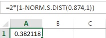
Thus, the p-value using EXCEL is 0.382, which is also same as the p-value obtained in chi-square test.
Thus, it is verified that
Want to see more full solutions like this?
Chapter 15 Solutions
APPLIED STAT.IN BUS.+ECONOMICS


- A marketing agency wants to determine whether different advertising platforms generate significantly different levels of customer engagement. The agency measures the average number of daily clicks on ads for three platforms: Social Media, Search Engines, and Email Campaigns. The agency collects data on daily clicks for each platform over a 10-day period and wants to test whether there is a statistically significant difference in the mean number of daily clicks among these platforms. Conduct ANOVA test. You can provide your answer by inserting a text box and the answer must include: also please provide a step by on getting the answers in excel Null hypothesis, Alternative hypothesis, Show answer (output table/summary table), and Conclusion based on the P value.arrow_forwardA company found that the daily sales revenue of its flagship product follows a normal distribution with a mean of $4500 and a standard deviation of $450. The company defines a "high-sales day" that is, any day with sales exceeding $4800. please provide a step by step on how to get the answers Q: What percentage of days can the company expect to have "high-sales days" or sales greater than $4800? Q: What is the sales revenue threshold for the bottom 10% of days? (please note that 10% refers to the probability/area under bell curve towards the lower tail of bell curve) Provide answers in the yellow cellsarrow_forwardBusiness Discussarrow_forward
- The following data represent total ventilation measured in liters of air per minute per square meter of body area for two independent (and randomly chosen) samples. Analyze these data using the appropriate non-parametric hypothesis testarrow_forwardeach column represents before & after measurements on the same individual. Analyze with the appropriate non-parametric hypothesis test for a paired design.arrow_forwardShould you be confident in applying your regression equation to estimate the heart rate of a python at 35°C? Why or why not?arrow_forward
 Big Ideas Math A Bridge To Success Algebra 1: Stu...AlgebraISBN:9781680331141Author:HOUGHTON MIFFLIN HARCOURTPublisher:Houghton Mifflin Harcourt
 Glencoe Algebra 1, Student Edition, 9780079039897...AlgebraISBN:9780079039897Author:CarterPublisher:McGraw Hill
 Holt Mcdougal Larson Pre-algebra: Student Edition...AlgebraISBN:9780547587776Author:HOLT MCDOUGALPublisher:HOLT MCDOUGAL