Chapter 15, Problem 15.69SE

a.

To determine

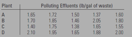
To check:whether the data present sufficient evidence to indicate a difference in the level of pollutants for the four different industrial plants.

Answer to Problem 15.69SE

Yes.

Explanation of Solution

Given:

Five samples of liquid waste were taken at the output of each four industrial plants.

The data is shown in the given below table

  

Calculation:

  $\begin{array}{l}\alpha =\text{significance level}=0.05\\ k=\text{Number of treatments}=4\\ n_1=\text{Sample size of first sample}=5\\ n_2=\text{Sample size of second sample}=5\\ n_3=\text{Sample size of third sample}=5\\ n_4=\text{Sample size of fourth sample}=8\\ n=n_1+n_2+n_3+n_4=5+5+5+5=20\end{array}$

Kruskal-Wallis test

The null hypothesis states that there is no difference between the population distribution. The alternatives hypothesis states the opposite of the null hypothesis.

  $\begin{array}{l}{H}_0:\text{ The population distributions are the same}\text{.}\\ H_1:\text{ atleast two of the population distributions differ in the location}\end{array}$

Determine the rank of every data value. The smallest value receives the rank 1, the second smallest value receives the rank 2, the third smallest value receives the rank 3, and so on. If multiple data values have the same value, then their rank is the average of the corresponding ranks.

The signed rank is the sign of the difference added to the rank.

Sample 1	Rank	Sample 2	Rank	Sample 3	Rank	Sample 4	Rank
1.65	9	1.7	11	1.4	3	2.1	20
1.72	12	1.85	15	1.75	13	1.95	17
1.5	5	1.46	4	1.38	2	1.65	16
1.37	1	2.05	19	1.65	9	1.88	9
1.6	7	1.8	14	1.55	6	2	18

Determine the sum of the ranks for each treatment:

  $\begin{array}{l}{T}_1=9+12+5+1+7\\ T_1=34\end{array}$

  $\begin{array}{l}{T}_2=11+15+4+19+14\\ T_2=63\end{array}$

  $\begin{array}{l}{T}_3=3+13+2+9+6\\ T_3=33\end{array}$

  $\begin{array}{l}{T}_4=20+17+9+16+18\\ T_4=80\end{array}$

Determine the value of the Kruskal-Wallis test statistics:

  $\begin{array}{l}H=\left(\frac{12}{bk\left(k+1\right)}{\displaystyle \sum _{i=1}^k\frac{T_i^2}{n_i}}\right)-3\left(n+1\right)\\ =\frac{12}{\left(20\right)\left(20\right)\left(20+1\right)}\left(\frac{{34}^2}{5}+\frac{{63}^2}{5}+\frac{{33}^2}{5}+\frac{{80}^2}{5}\right)-3\left(20+1\right)\\ \approx 9.08\end{array}$

The $P\text{-value}$ is the probability of obtaining a value of the test statistics, or a value more extreme. The $P\text{-value}$ is the number in the common title of chi-square distribution table in the appendix containing the $x^2$ value in the row $df=k-1=4-1=3$ :

  $0.025<P<0.05$

If the $P\text{-value}$ is less than the significance level $\alpha$ , then rejected the null hypothesis:

  $P<0.05\Rightarrow \text{Reject }{H}_0$

There is sufficient evidence to support the claim that there is a difference in a level of pollutants for the four industrial plants.

b.

To determine

To find:the approximate p-value for the test and interpret its value.

Answer to Problem 15.69SE

  $0.025<P<0.05$

Explanation of Solution

Given:

Five samples of liquid waste were taken at the output of each four industrial plants.

The data is shown in the given below table

  

Calculation:

  $\begin{array}{l}\alpha =\text{significance level}=0.05\\ k=\text{Number of treatments}=4\\ n_1=\text{Sample size of first sample}=5\\ n_2=\text{Sample size of second sample}=5\\ n_3=\text{Sample size of third sample}=5\\ n_4=\text{Sample size of fourth sample}=8\\ n=n_1+n_2+n_3+n_4=5+5+5+5=20\end{array}$

Kruskal-Wallis test

The null hypothesis states that there is no difference between the population distribution. The alternatives hypothesis states the opposite of the null hypothesis.

  $\begin{array}{l}{H}_0:\text{ The population distributions are the same}\text{.}\\ H_1:\text{ atleast two of the population distributions differ in the location}\end{array}$

Determine the rank of every data value. The smallest value receives the rank 1, the second smallest value receives the rank 2, the third smallest value receives the rank 3, and so on. If multiple data values have the same value, then their rank is the average of the corresponding ranks.

The signed rank is the sign of the difference added to the rank.

Sample 1	Rank	Sample 2	Rank	Sample 3	Rank	Sample 4	Rank
1.65	9	1.7	11	1.4	3	2.1	20
1.72	12	1.85	15	1.75	13	1.95	17
1.5	5	1.46	4	1.38	2	1.65	16
1.37	1	2.05	19	1.65	9	1.88	9
1.6	7	1.8	14	1.55	6	2	18

Determine the sum of the ranks for each treatment:

  $\begin{array}{l}{T}_1=9+12+5+1+7\\ T_1=34\end{array}$

  $\begin{array}{l}{T}_2=11+15+4+19+14\\ T_2=63\end{array}$

  $\begin{array}{l}{T}_3=3+13+2+9+6\\ T_3=33\end{array}$

  $\begin{array}{l}{T}_4=20+17+9+16+18\\ T_4=80\end{array}$

Determine the value of the Kruskal-Wallis test statistics:

  $\begin{array}{l}H=\left(\frac{12}{bk\left(k+1\right)}{\displaystyle \sum _{i=1}^k\frac{T_i^2}{n_i}}\right)-3\left(n+1\right)\\ =\frac{12}{\left(20\right)\left(20\right)\left(20+1\right)}\left(\frac{{34}^2}{5}+\frac{{63}^2}{5}+\frac{{33}^2}{5}+\frac{{80}^2}{5}\right)-3\left(20+1\right)\\ \approx 9.08\end{array}$

c.

To determine

To compare: the test result in part (a) with the analysis of variance test.

Answer to Problem 15.69SE

Yes.

Explanation of Solution

Given:

Five samples of liquid waste were taken at the output of each four industrial plants.

The data is shown in the given below table

  

Calculation:

The null hypothesis states that there is all population means are equal

  $H_0:{\mu }_1={\mu }_2={\mu }_3={\mu }_4$

The alternative hypothesis states the opposite of the null hypothesis:

  $H_1:\text{ At least one of the population means is difference from the others}$

Let us determine the necessary sums:

  $\begin{array}{l}{\displaystyle \sum x_1}=1.65+1.72+1.5+1.37+1.6=7.84\\ {\displaystyle \sum x_2}=1.70+1.85+1.46+2.05+1.80=8.86\\ {\displaystyle \sum x_3}=1.40+1.75+1.38+1.65+1.55=7.73\\ {\displaystyle \sum x_4}=2.10+1.95+1.65+1.88+2.00=9.58\end{array}$

  $\begin{array}{l}{\displaystyle \sum x}={\displaystyle \sum x_1}+{\displaystyle \sum x_2+{\displaystyle \sum x_3}}+{\displaystyle \sum x_4}\\ =7.84+8.86+7.73+9.58\\ =34.01\end{array}$

  $\begin{array}{l}{{\displaystyle \sum x}}^2={1.65}^2+{1.72}^2+{1.5}^2+{1.37}^2+{1.6}^2\\ +{1.70}^2+{1.85}^2+{1.46}^2+{2.05}^2+{1.80}^2\\ +{1.40}^2+{1.75}^2+{1.38}^2+{1.65}^2+{1.55}^2\\ +{2.10}^2+{1.95}^2+{1.65}^2+{1.88}^2+{2.00}^2\\ =58.7757\end{array}$

Determine the value of total-group variability. Total $SS:$

Total $SS={{\displaystyle \sum x}}^2-\frac{{\left({\displaystyle \sum x}\right)}^2}{n}=58.7757-\frac{{34.01}^2}{20}\approx 0.941695$

Determine the value of the sum of the square of the square between groups:

  $\begin{array}{l}SST={\displaystyle \sum _{allgroups}\frac{{\displaystyle \sum x_i}}{n_i}}-\frac{{\left({\displaystyle \sum x}\right)}^2}{n}\\ =\left(\frac{{7.84}^2}{5}+\frac{{8.86}^2}{5}+\frac{{7.73}^2}{5}+\frac{{9.58}^2}{5}\right)-\frac{{34.01}^2}{20}\\ \approx 0.464895\end{array}$

The value of the sum of squares within groups is then the value of the total group variability decreased by the value of the sum of the square between groups.

Total $SS=SST+SSE\text{ holds}$ :

  $SSE=\text{Total }SS-SST=0.941695-0.464895=0.4768$

  $d{f}_T$ is the number of groups $k$ decreases by 1,$d{f}_T=k-1=4-1=3$

  $d{f}_E$ is the total sample sized decreases by number of groups $k$ ,

  $d{f}_E=n-k=20-4=16$

Total $df$ is the sum of separate degree of freedom $d{f}_T$ and $d{f}_E$ .

  $MST$ is $SST$ dived by $d{f}_T$ :

  $MST=\frac{SST}{d{f}_T}=\frac{0.464895}{3}=0.154965$

  $MSE$ is $SSE$ dived by $d{f}_T$ :

  $MSE=\frac{SSE}{d{f}_E}=\frac{0.4768}{16}=0.0298$

The value of the test statistic F is then $MST$ divided by $MSE$ .

  $F=\frac{MST}{MSE}=\frac{0.154965}{0.0298}\approx 5.2$

Combine the information in an ANOVA table:

Source	df	SS	MS	F
Treatments	3	0.464895	0.154965	5.2
Error	16	0.4768	0.0298
Total	19	0.941695

The $P\text{-value}$ is the probability of obtaining a value of the test statistics, or a value more extreme. The $P\text{-value}$ is the number in the row title of F-distribution table in the appendix containing the $x^2$ value in the row $d{f}_2=d{f}_3=16\text{ and }d{f}_1=d{f}_T=3$ :

  $0.01<P<0.025$

If the $P\text{-value}$ is less than the significance level $\alpha$ , then rejected the null hypothesis:

  $P<0.05\Rightarrow \text{Reject }{H}_0$

There is sufficient evidence to support the claim that there is a difference in the mean amounts of effluents discharged by the four plants.