
Videos
a.
Test for main effects and interactions at
a.
Answer to Problem 75SE
Main effect of factor A is significant.
Main effect of factor B is not significant.
The interaction is significant.
Explanation of Solution
Calculation:
The data represents the two factorial experiments to investigate the effect of pH and catalyst concentration on product viscosity.
Factor A is pH and Factor B is Catalyst Concentration.
State the hypotheses:
Main effect of factor A:
Null hypothesis:
Alternative hypothesis:
Main effect of factor B:
Null hypothesis:
Alternative hypothesis:
Interaction effect of Factor A and B:
Null hypothesis:
Alternative hypothesis:
Step-by-step procedure to find the factorial design table is as follows:
Software procedure:
- Choose Stat > DOE > Factorial > Create Factorial Design.
- Under Type of Design, choose General full factorial design.
- From Number of factors, choose 2.
- Click Designs.
- In Factor A, type A under Name and type 2 Under Number of Levels.
- In Factor B, type B under Name and type 2 Under Number of Levels.
- From Number of replicates, choose 4.
- Click OK.
- Select Summary table under Results.
- Click OK.
- Enter the corresponding response in the newly created factorial design worksheet.
Step-by-step procedure for finding the ANOVA table is as follows:
- Choose Stat > DOE > Factorial > Analyze Factorial Design.
- In Response, enter Responses.
- In Terms, select all the terms.
- In Results, choose “Model summary and ANOVA table”.
- Click OK in all the dialog boxes.
Output obtained by MINITAB procedure is as follows:
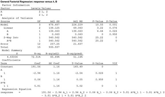
For Factor A, the F-test statistic is 6.44 and the p-value is 0.026.
For Factor B, the F-test statistic is 0.00 and the p-value is 0.958.
For interaction, the F-test statistic is 25.22 and the p-value is 0.00.
Decision:
If
If
Conclusion:
Factor A:
Here, the P-value is less than the level of significance.
That is,
Therefore, the null hypothesis is rejected.
Thus, Main effect of factor A is significant at
Factor B:
Here, the P-value is greater than the level of significance.
That is,
Therefore, the null hypothesis is not rejected.
Thus, Main effect of factor B is not significant at
Interaction:
Here, the P-value is less than the level of significance.
That is,
Therefore, the null hypothesis is rejected.
Thus, the interaction is significant at
Thus, it can be concluded that:
Main effect of factor A is significant.
Main effect of factor B is not significant.
The interaction is significant.
b.
Graphically analyze the interaction.
b.
Answer to Problem 75SE
The interaction plot indicates that there is a strong interaction.
Explanation of Solution
Calculation:
Software procedure:
Step by step procedure to obtain normal plot and residual plot using Minitab software is given as,
- Choose Stat > DOE > Factorial > Factorial plot.
- In Interaction select setup.
- In Response, enter Responses.
- In Factor included plots, select AA,BB.
- In Types of means to use in plot, choose Data means..
- Click OK.
Output using the MINITAB software is given below:
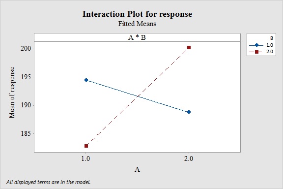
Interpretation:
From the interaction plot it is clear that when Factor A is at low level, the response is large for the lower values of B and is small at the high level of B. Similarly, if Factor A is at high level, the response is small for the higher values of B and is higher at the smallest level of B.
Thus, the interaction plot indicates that there is a strong interaction.
c.
Analyze the residuals from the experiment.
c.
Answer to Problem 75SE
The residuals are acceptable and normality assumption is not reasonable.
Explanation of Solution
Justification:
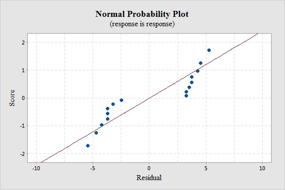
The conditions for a residual plot and normal plot that is well fitted for the data are,
- There should not any bend, which would violate the straight enough condition.
- There must not any outlier, which, were not clear before.
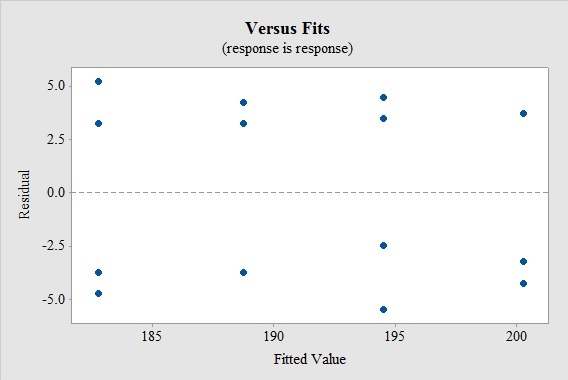
- There should not any change in the spread of the residuals from one part to another part of the plot.
Software procedure:
Step by step procedure to obtain normal plot and residual plot using Minitab software is given as,
- Choose Stat > DOE > Factorial > Analyze Factorial Design.
- In Response, enter Responses.
- In Terms, select all the terms.
- In Results, choose “Model summary and ANOVA table”.
- In Confidence level, enter 0.95.
- In residual plots select Normal plot of residuals, Residual versus fits.
- In residual versus the variables enter the column of Factor A and Factor B.
- Click OK.
Output using the MINITAB software is given below:
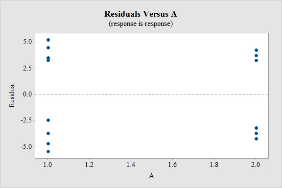
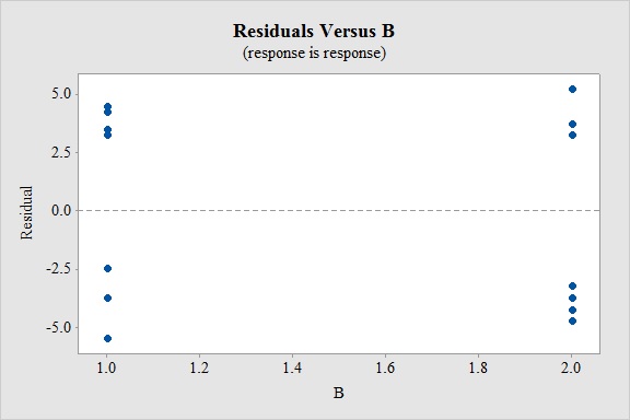
Interpretation:
In normal probability plot, the points do not lie along the straight line and there is a gap in the middle of the normal probability plot. Thus, normality assumption is not satisfied. There is no much variability for the variables.
Also, there is no change in the spread of the residuals from one part to another part of the residual plot.
Thus, the residuals are acceptable and normality assumption is not reasonable.
Want to see more full solutions like this?
Chapter 14 Solutions
Applied Statistics and Probability for Engineers


- The PDF of an amplitude X of a Gaussian signal x(t) is given by:arrow_forwardThe PDF of a random variable X is given by the equation in the picture.arrow_forwardFor a binary asymmetric channel with Py|X(0|1) = 0.1 and Py|X(1|0) = 0.2; PX(0) = 0.4 isthe probability of a bit of “0” being transmitted. X is the transmitted digit, and Y is the received digit.a. Find the values of Py(0) and Py(1).b. What is the probability that only 0s will be received for a sequence of 10 digits transmitted?c. What is the probability that 8 1s and 2 0s will be received for the same sequence of 10 digits?d. What is the probability that at least 5 0s will be received for the same sequence of 10 digits?arrow_forward
- V2 360 Step down + I₁ = I2 10KVA 120V 10KVA 1₂ = 360-120 or 2nd Ratio's V₂ m 120 Ratio= 360 √2 H I2 I, + I2 120arrow_forwardQ2. [20 points] An amplitude X of a Gaussian signal x(t) has a mean value of 2 and an RMS value of √(10), i.e. square root of 10. Determine the PDF of x(t).arrow_forwardIn a network with 12 links, one of the links has failed. The failed link is randomlylocated. An electrical engineer tests the links one by one until the failed link is found.a. What is the probability that the engineer will find the failed link in the first test?b. What is the probability that the engineer will find the failed link in five tests?Note: You should assume that for Part b, the five tests are done consecutively.arrow_forward
- Problem 3. Pricing a multi-stock option the Margrabe formula The purpose of this problem is to price a swap option in a 2-stock model, similarly as what we did in the example in the lectures. We consider a two-dimensional Brownian motion given by W₁ = (W(¹), W(2)) on a probability space (Q, F,P). Two stock prices are modeled by the following equations: dX = dY₁ = X₁ (rdt+ rdt+0₁dW!) (²)), Y₁ (rdt+dW+0zdW!"), with Xo xo and Yo =yo. This corresponds to the multi-stock model studied in class, but with notation (X+, Y₁) instead of (S(1), S(2)). Given the model above, the measure P is already the risk-neutral measure (Both stocks have rate of return r). We write σ = 0₁+0%. We consider a swap option, which gives you the right, at time T, to exchange one share of X for one share of Y. That is, the option has payoff F=(Yr-XT). (a) We first assume that r = 0 (for questions (a)-(f)). Write an explicit expression for the process Xt. Reminder before proceeding to question (b): Girsanov's theorem…arrow_forwardProblem 1. Multi-stock model We consider a 2-stock model similar to the one studied in class. Namely, we consider = S(1) S(2) = S(¹) exp (σ1B(1) + (M1 - 0/1 ) S(²) exp (02B(2) + (H₂- M2 where (B(¹) ) +20 and (B(2) ) +≥o are two Brownian motions, with t≥0 Cov (B(¹), B(2)) = p min{t, s}. " The purpose of this problem is to prove that there indeed exists a 2-dimensional Brownian motion (W+)+20 (W(1), W(2))+20 such that = S(1) S(2) = = S(¹) exp (011W(¹) + (μ₁ - 01/1) t) 롱) S(²) exp (021W (1) + 022W(2) + (112 - 03/01/12) t). where σ11, 21, 22 are constants to be determined (as functions of σ1, σ2, p). Hint: The constants will follow the formulas developed in the lectures. (a) To show existence of (Ŵ+), first write the expression for both W. (¹) and W (2) functions of (B(1), B(²)). as (b) Using the formulas obtained in (a), show that the process (WA) is actually a 2- dimensional standard Brownian motion (i.e. show that each component is normal, with mean 0, variance t, and that their…arrow_forwardThe scores of 8 students on the midterm exam and final exam were as follows. Student Midterm Final Anderson 98 89 Bailey 88 74 Cruz 87 97 DeSana 85 79 Erickson 85 94 Francis 83 71 Gray 74 98 Harris 70 91 Find the value of the (Spearman's) rank correlation coefficient test statistic that would be used to test the claim of no correlation between midterm score and final exam score. Round your answer to 3 places after the decimal point, if necessary. Test statistic: rs =arrow_forward
- Business discussarrow_forwardBusiness discussarrow_forwardI just need to know why this is wrong below: What is the test statistic W? W=5 (incorrect) and What is the p-value of this test? (p-value < 0.001-- incorrect) Use the Wilcoxon signed rank test to test the hypothesis that the median number of pages in the statistics books in the library from which the sample was taken is 400. A sample of 12 statistics books have the following numbers of pages pages 127 217 486 132 397 297 396 327 292 256 358 272 What is the sum of the negative ranks (W-)? 75 What is the sum of the positive ranks (W+)? 5What type of test is this? two tailedWhat is the test statistic W? 5 These are the critical values for a 1-tailed Wilcoxon Signed Rank test for n=12 Alpha Level 0.001 0.005 0.01 0.025 0.05 0.1 0.2 Critical Value 75 70 68 64 60 56 50 What is the p-value for this test? p-value < 0.001arrow_forward
 MATLAB: An Introduction with ApplicationsStatisticsISBN:9781119256830Author:Amos GilatPublisher:John Wiley & Sons Inc
 Probability and Statistics for Engineering and th...StatisticsISBN:9781305251809Author:Jay L. DevorePublisher:Cengage Learning
 Statistics for The Behavioral Sciences (MindTap C...StatisticsISBN:9781305504912Author:Frederick J Gravetter, Larry B. WallnauPublisher:Cengage Learning
 Elementary Statistics: Picturing the World (7th E...StatisticsISBN:9780134683416Author:Ron Larson, Betsy FarberPublisher:PEARSON
 The Basic Practice of StatisticsStatisticsISBN:9781319042578Author:David S. Moore, William I. Notz, Michael A. FlignerPublisher:W. H. Freeman
 Introduction to the Practice of StatisticsStatisticsISBN:9781319013387Author:David S. Moore, George P. McCabe, Bruce A. CraigPublisher:W. H. Freeman