STATISTICS F/BUS.+ECON-W/ACCESS>CUSTOM<
18th Edition
ISBN: 9781323751503
Author: MCCLAVE
Publisher: PEARSON C
expand_more
expand_more
format_list_bulleted
Videos
Textbook Question
Chapter 14, Problem 14.60ACB
Retail prices of food items. In 1990, the average weekly food cost for a suburban family of four was estimated to be $154.40. The table (next column) presents the retail prices of four food items for selected years from 1990 to 2015. Assume a typical suburban family of four purchased the following quantities of food, on average, each week during 1990:
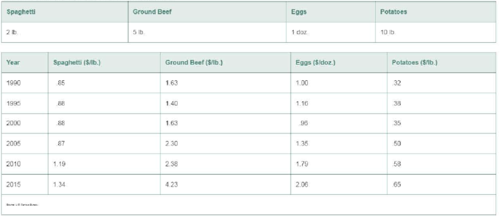
a. Calculate a Laspeyres price index for 1990 to 2015, using 1990 as the base year.
b. According to your index, how much did the above “basket” of foods increase or decrease in price from 1990 to 2015?
Expert Solution & Answer
Want to see the full answer?
Check out a sample textbook solution
Students have asked these similar questions
Find binomial probability if:
x = 8, n = 10, p = 0.7
x= 3, n=5, p = 0.3
x = 4, n=7, p = 0.6
Quality Control: A factory produces light bulbs with a 2% defect rate. If a random sample of 20 bulbs is tested, what is the probability that exactly 2 bulbs are defective? (hint: p=2% or 0.02; x =2, n=20; use the same logic for the following problems)
Marketing Campaign: A marketing company sends out 1,000 promotional emails. The probability of any email being opened is 0.15. What is the probability that exactly 150 emails will be opened? (hint: total emails or n=1000, x =150)
Customer Satisfaction: A survey shows that 70% of customers are satisfied with a new product. Out of 10 randomly selected customers, what is the probability that at least 8 are satisfied? (hint: One of the keyword in this question is “at least 8”, it is not “exactly 8”, the correct formula for this should be = 1- (binom.dist(7, 10, 0.7, TRUE)). The part in the princess will give you the probability of seven and less than…
please answer these questions
Selon une économiste d’une société financière, les dépenses moyennes pour « meubles et appareils de maison » ont été moins importantes pour les ménages de la région de Montréal, que celles de la région de Québec.
Un échantillon aléatoire de 14 ménages pour la région de Montréal et de 16 ménages pour la région Québec est tiré et donne les données suivantes, en ce qui a trait aux dépenses pour ce secteur d’activité économique.
On suppose que les données de chaque population sont distribuées selon une loi normale.
Nous sommes intéressé à connaitre si les variances des populations sont égales.a) Faites le test d’hypothèse sur deux variances approprié au seuil de signification de 1 %. Inclure les informations suivantes :
i. Hypothèse / Identification des populationsii. Valeur(s) critique(s) de Fiii. Règle de décisioniv. Valeur du rapport Fv. Décision et conclusion
b) A partir des résultats obtenus en a), est-ce que l’hypothèse d’égalité des variances pour cette…
Chapter 14 Solutions
STATISTICS F/BUS.+ECON-W/ACCESS>CUSTOM<
Ch. 14.1 - Explain in words how to construct a simple index.Ch. 14.1 - Explain in words how to calculate the following...Ch. 14.1 - Explain in words the difference between Laspeyres...Ch. 14.1 - The table below gives the prices for three...Ch. 14.1 - Refer to Exercise 14.4. The next table gives the...Ch. 14.1 - Annual median family income. The table below lists...Ch. 14.1 - Annual U.S. craft beer production. While overall...Ch. 14.1 - Quarterly single-family housing starts. The...Ch. 14.1 - Spot price of natural gas. The table shown in the...Ch. 14.1 - Employment in farm and nonfarm categories....
Ch. 14.1 - GOP personal consumption expenditures. The gross...Ch. 14.1 - GDP personal consumption expenditures (contd)....Ch. 14.1 - Weekly earnings for workers. The table in the next...Ch. 14.1 - Production and price of metals. The level or price...Ch. 14.2 - Describe the effect of selecting an exponential...Ch. 14.2 - A monthly time series is shown in the table to the...Ch. 14.2 - Annual U.S. craft beer production. Refer to the...Ch. 14.2 - Foreign fish production. Overfishing and pollution...Ch. 14.2 - Yearly price of gold. The price of gold is used by...Ch. 14.2 - Personal consumption in transportation. There has...Ch. 14.2 - OPEC crude oil imports. The data in the table...Ch. 14.2 - SP 500 Stock Index. Standard Poors 500 Composite...Ch. 14.5 - How does the choice of the smoothing constant w...Ch. 14.5 - Refer to Exercise 14.4 (p. 14-9). The table with...Ch. 14.5 - Annual U.S. craft beer production. Refer to...Ch. 14.5 - Quarterly single-family housing starts. Refer to...Ch. 14.5 - Consumer Price Index. The CPI measures the...Ch. 14.5 - OPEC crude oil imports. Refer to the annual OPEC...Ch. 14.5 - SP 500 Stock Index. Refer to the quarterly...Ch. 14.5 - SP 500 Stock Index (contd). Refer to Exercise...Ch. 14.5 - Monthly gold prices. The fluctuation of gold...Ch. 14.6 - Annual U.S. craft beer production. Refer to the...Ch. 14.6 - Annual U.S. craft beer production (contd). Refer...Ch. 14.6 - SP 500 Stock Index. Refer to your exponential...Ch. 14.6 - SP 500 Stock Index (contd). Refer to your Holt...Ch. 14.6 - Monthly gold prices. Refer to the monthly gold...Ch. 14.6 - US school enrollments. The next table reports...Ch. 14.8 - The annual price of a finished product (in cents...Ch. 14.8 - Retail sales in Quarters 14 over a 10-year period...Ch. 14.8 - What advantage do regression forecasts have over...Ch. 14.8 - Mortgage interest rates. The level at which...Ch. 14.8 - Price of natural gas. Refer to Exercise 14.9 (p....Ch. 14.8 - A gasoline tax on carbon emissions. In an effort...Ch. 14.8 - Predicting presidential elections. Researchers at...Ch. 14.8 - Life insurance policies in force. The table below...Ch. 14.8 - Graphing calculator sales. The next table presents...Ch. 14.8 - Prob. 14.47ACICh. 14.9 - Define autocorrelation. Explain why it is...Ch. 14.9 - For each case, indicate the decision regarding the...Ch. 14.9 - What do the following Durbin-Watson statistics...Ch. 14.9 - Company donations to charity. Refer to the Journal...Ch. 14.9 - Forecasting monthly car and truck sales. Forecasts...Ch. 14.9 - Predicting presidential elections. Refer to the...Ch. 14.9 - Mortgage interest rates. Refer to the data on...Ch. 14.9 - Price of natural gas. Refer to the annual data on...Ch. 14.9 - Life insurance policies in force. Refer to the...Ch. 14.9 - Modeling the deposit share of a retail bank....Ch. 14 - Insured Social Security workers. Workers insured...Ch. 14 - Insured Social Security workers (contd). Refer to...Ch. 14 - Retail prices of food items. In 1990, the average...Ch. 14 - Demand for emergency room services. With the...Ch. 14 - Mortgage interest rates. Refer to the annual...Ch. 14 - Price of Abbott Labs stock. The yearly closing...Ch. 14 - Price o f Abbott Labs stock (contd). Refer to...Ch. 14 - Prob. 14.65ACICh. 14 - Prob. 14.66ACICh. 14 - Quarterly GOP values (contd). Refer to Exercise...Ch. 14 - Prob. 14.68ACICh. 14 - Prob. 14.69ACICh. 14 - Prob. 14.70ACICh. 14 - IBM stock prices. Refer to Example 14.1 (p. 14-5)...Ch. 14 - Prob. 14.72ACI
Knowledge Booster


Learn more about
Need a deep-dive on the concept behind this application? Look no further. Learn more about this topic, statistics and related others by exploring similar questions and additional content below.Similar questions
- According to an economist from a financial company, the average expenditures on "furniture and household appliances" have been lower for households in the Montreal area than those in the Quebec region. A random sample of 14 households from the Montreal region and 16 households from the Quebec region was taken, providing the following data regarding expenditures in this economic sector. It is assumed that the data from each population are distributed normally. We are interested in knowing if the variances of the populations are equal. a) Perform the appropriate hypothesis test on two variances at a significance level of 1%. Include the following information: i. Hypothesis / Identification of populations ii. Critical F-value(s) iii. Decision rule iv. F-ratio value v. Decision and conclusion b) Based on the results obtained in a), is the hypothesis of equal variances for this socio-economic characteristic measured in these two populations upheld? c) Based on the results obtained in a),…arrow_forwardA major company in the Montreal area, offering a range of engineering services from project preparation to construction execution, and industrial project management, wants to ensure that the individuals who are responsible for project cost estimation and bid preparation demonstrate a certain uniformity in their estimates. The head of civil engineering and municipal services decided to structure an experimental plan to detect if there could be significant differences in project evaluation. Seven projects were selected, each of which had to be evaluated by each of the two estimators, with the order of the projects submitted being random. The obtained estimates are presented in the table below. a) Complete the table above by calculating: i. The differences (A-B) ii. The sum of the differences iii. The mean of the differences iv. The standard deviation of the differences b) What is the value of the t-statistic? c) What is the critical t-value for this test at a significance level of 1%?…arrow_forwardCompute the relative risk of falling for the two groups (did not stop walking vs. did stop). State/interpret your result verbally.arrow_forward
- Microsoft Excel include formulasarrow_forwardQuestion 1 The data shown in Table 1 are and R values for 24 samples of size n = 5 taken from a process producing bearings. The measurements are made on the inside diameter of the bearing, with only the last three decimals recorded (i.e., 34.5 should be 0.50345). Table 1: Bearing Diameter Data Sample Number I R Sample Number I R 1 34.5 3 13 35.4 8 2 34.2 4 14 34.0 6 3 31.6 4 15 37.1 5 4 31.5 4 16 34.9 7 5 35.0 5 17 33.5 4 6 34.1 6 18 31.7 3 7 32.6 4 19 34.0 8 8 33.8 3 20 35.1 9 34.8 7 21 33.7 2 10 33.6 8 22 32.8 1 11 31.9 3 23 33.5 3 12 38.6 9 24 34.2 2 (a) Set up and R charts on this process. Does the process seem to be in statistical control? If necessary, revise the trial control limits. [15 pts] (b) If specifications on this diameter are 0.5030±0.0010, find the percentage of nonconforming bearings pro- duced by this process. Assume that diameter is normally distributed. [10 pts] 1arrow_forward4. (5 pts) Conduct a chi-square contingency test (test of independence) to assess whether there is an association between the behavior of the elderly person (did not stop to talk, did stop to talk) and their likelihood of falling. Below, please state your null and alternative hypotheses, calculate your expected values and write them in the table, compute the test statistic, test the null by comparing your test statistic to the critical value in Table A (p. 713-714) of your textbook and/or estimating the P-value, and provide your conclusions in written form. Make sure to show your work. Did not stop walking to talk Stopped walking to talk Suffered a fall 12 11 Totals 23 Did not suffer a fall | 2 Totals 35 37 14 46 60 Tarrow_forward
- Question 2 Parts manufactured by an injection molding process are subjected to a compressive strength test. Twenty samples of five parts each are collected, and the compressive strengths (in psi) are shown in Table 2. Table 2: Strength Data for Question 2 Sample Number x1 x2 23 x4 x5 R 1 83.0 2 88.6 78.3 78.8 3 85.7 75.8 84.3 81.2 78.7 75.7 77.0 71.0 84.2 81.0 79.1 7.3 80.2 17.6 75.2 80.4 10.4 4 80.8 74.4 82.5 74.1 75.7 77.5 8.4 5 83.4 78.4 82.6 78.2 78.9 80.3 5.2 File Preview 6 75.3 79.9 87.3 89.7 81.8 82.8 14.5 7 74.5 78.0 80.8 73.4 79.7 77.3 7.4 8 79.2 84.4 81.5 86.0 74.5 81.1 11.4 9 80.5 86.2 76.2 64.1 80.2 81.4 9.9 10 75.7 75.2 71.1 82.1 74.3 75.7 10.9 11 80.0 81.5 78.4 73.8 78.1 78.4 7.7 12 80.6 81.8 79.3 73.8 81.7 79.4 8.0 13 82.7 81.3 79.1 82.0 79.5 80.9 3.6 14 79.2 74.9 78.6 77.7 75.3 77.1 4.3 15 85.5 82.1 82.8 73.4 71.7 79.1 13.8 16 78.8 79.6 80.2 79.1 80.8 79.7 2.0 17 82.1 78.2 18 84.5 76.9 75.5 83.5 81.2 19 79.0 77.8 20 84.5 73.1 78.2 82.1 79.2 81.1 7.6 81.2 84.4 81.6 80.8…arrow_forwardName: Lab Time: Quiz 7 & 8 (Take Home) - due Wednesday, Feb. 26 Contingency Analysis (Ch. 9) In lab 5, part 3, you will create a mosaic plot and conducted a chi-square contingency test to evaluate whether elderly patients who did not stop walking to talk (vs. those who did stop) were more likely to suffer a fall in the next six months. I have tabulated the data below. Answer the questions below. Please show your calculations on this or a separate sheet. Did not stop walking to talk Stopped walking to talk Totals Suffered a fall Did not suffer a fall Totals 12 11 23 2 35 37 14 14 46 60 Quiz 7: 1. (2 pts) Compute the odds of falling for each group. Compute the odds ratio for those who did not stop walking vs. those who did stop walking. Interpret your result verbally.arrow_forwardSolve please and thank you!arrow_forward
- 7. In a 2011 article, M. Radelet and G. Pierce reported a logistic prediction equation for the death penalty verdicts in North Carolina. Let Y denote whether a subject convicted of murder received the death penalty (1=yes), for the defendant's race h (h1, black; h = 2, white), victim's race i (i = 1, black; i = 2, white), and number of additional factors j (j = 0, 1, 2). For the model logit[P(Y = 1)] = a + ß₁₂ + By + B²², they reported = -5.26, D â BD = 0, BD = 0.17, BY = 0, BY = 0.91, B = 0, B = 2.02, B = 3.98. (a) Estimate the probability of receiving the death penalty for the group most likely to receive it. [4 pts] (b) If, instead, parameters used constraints 3D = BY = 35 = 0, report the esti- mates. [3 pts] h (c) If, instead, parameters used constraints Σ₁ = Σ₁ BY = Σ; B = 0, report the estimates. [3 pts] Hint the probabilities, odds and odds ratios do not change with constraints.arrow_forwardSolve please and thank you!arrow_forwardSolve please and thank you!arrow_forward
arrow_back_ios
SEE MORE QUESTIONS
arrow_forward_ios
Recommended textbooks for you
 Holt Mcdougal Larson Pre-algebra: Student Edition...AlgebraISBN:9780547587776Author:HOLT MCDOUGALPublisher:HOLT MCDOUGAL
 Algebra: Structure And Method, Book 1AlgebraISBN:9780395977224Author:Richard G. Brown, Mary P. Dolciani, Robert H. Sorgenfrey, William L. ColePublisher:McDougal Littell
 Elementary Geometry For College Students, 7eGeometryISBN:9781337614085Author:Alexander, Daniel C.; Koeberlein, Geralyn M.Publisher:Cengage,
Holt Mcdougal Larson Pre-algebra: Student Edition...
Algebra
ISBN:9780547587776
Author:HOLT MCDOUGAL
Publisher:HOLT MCDOUGAL
Algebra: Structure And Method, Book 1
Algebra
ISBN:9780395977224
Author:Richard G. Brown, Mary P. Dolciani, Robert H. Sorgenfrey, William L. Cole
Publisher:McDougal Littell
Elementary Geometry For College Students, 7e
Geometry
ISBN:9781337614085
Author:Alexander, Daniel C.; Koeberlein, Geralyn M.
Publisher:Cengage,
Time Series Analysis Theory & Uni-variate Forecasting Techniques; Author: Analytics University;https://www.youtube.com/watch?v=_X5q9FYLGxM;License: Standard YouTube License, CC-BY
Operations management 101: Time-series, forecasting introduction; Author: Brandoz Foltz;https://www.youtube.com/watch?v=EaqZP36ool8;License: Standard YouTube License, CC-BY