Concept explainers
Videos
a.
To find:The regression equation for the data.
a.
Answer to Problem 21E
The regression equation for the data is
Explanation of Solution
Given information: The data is shown below.
| 31.3 | 50 | 19 | 4.0 | 37.4 | 60 | 30 | 5.0 | 24.0 | 60 | 24 | 4.0 | 51.0 | 80 | 34 | 7.5 |
| 56.9 | 90 | 38 | 8.0 | 43.3 | 60 | 26 | 7.0 | 36.2 | 50 | 21 | 7.0 | 34.3 | 60 | 22 | 2.5 |
| 43.1 | 70 | 28 | 6.5 | 36.3 | 70 | 25 | 7.5 | 26.5 | 50 | 17 | 2.0 | 31.5 | 60 | 24 | 5.0 |
| 41.5 | 70 | 25 | 5.5 | 38.4 | 70 | 31 | 5.5 | 47.1 | 80 | 34 | 8.5 | 33.2 | 60 | 23 | 4.0 |
| 39.0 | 60 | 26 | 6.5 | 41.5 | 60 | 27 | 7.5 | 38.1 | 70 | 27 | 5.5 | 39.2 | 60 | 29 | 6.5 |
| 40.9 | 70 | 29 | 5.0 | 36.l | 60 | 23 | 6.0 | 33.5 | 60 | 24 | 2.5 | 46.7 | 70 | 27 | 7.5 |
| 35.9 | 60 | 23 | 5.5 | 38.5 | 60 | 23 | 6.0 | 43.6 | 70 | 27 | 10.0 | 30.4 | 70 | 32 | 4.0 |
| 43.5 | 70 | 28 | 5.5 | 42.4 | 60 | 24 | 9.0 | 41.0 | 80 | 32 | 6.5 | 43.2 | 60 | 25 | 5.5 |
| 47.9 | 80 | 34 | 6.5 | 46.5 | 70 | 31 | 5.5 | 50.2 | 50 | 26 | 9.0 | 30.6 | 60 | 26 | 3.5 |
| 33.8 | 70 | 26 | 4.5 | 43.1 | 80 | 32 | 6.0 | 34.4 | 50 | 22 | 4.0 | 43.3 | 70 | 28 | 7.5 |
| 41.1 | 70 | 26 | 8.0 | 50.8 | 60 | 26 | 10.0 | 47.9 | 80 | 34 | 6.5 | 32.4 | 60 | 22 | 5.5 |
| 38.7 | 70 | 26 | 8.0 | 44.2 | 70 | 28 | 4.5 | 46.2 | 50 | 21 | 10.0 | 35.5 | 60 | 22 | 4.5 |
Calculation:
The MINITAB is shown below,
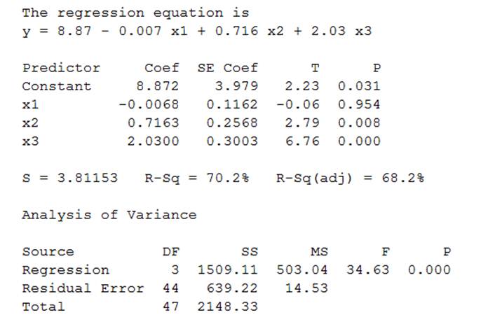
Figure-1
From Figure-1 it is clear that the regression equation is
b.
To find: The value of variable
b.
Answer to Problem 21E
The value of variable
Explanation of Solution
Given information: The data is shown below.
| 31.3 | 50 | 19 | 4.0 | 37.4 | 60 | 30 | 5.0 | 24.0 | 60 | 24 | 4.0 | 51.0 | 80 | 34 | 7.5 |
| 56.9 | 90 | 38 | 8.0 | 43.3 | 60 | 26 | 7.0 | 36.2 | 50 | 21 | 7.0 | 34.3 | 60 | 22 | 2.5 |
| 43.1 | 70 | 28 | 6.5 | 36.3 | 70 | 25 | 7.5 | 26.5 | 50 | 17 | 2.0 | 31.5 | 60 | 24 | 5.0 |
| 41.5 | 70 | 25 | 5.5 | 38.4 | 70 | 31 | 5.5 | 47.1 | 80 | 34 | 8.5 | 33.2 | 60 | 23 | 4.0 |
| 39.0 | 60 | 26 | 6.5 | 41.5 | 60 | 27 | 7.5 | 38.1 | 70 | 27 | 5.5 | 39.2 | 60 | 29 | 6.5 |
| 40.9 | 70 | 29 | 5.0 | 36.l | 60 | 23 | 6.0 | 33.5 | 60 | 24 | 2.5 | 46.7 | 70 | 27 | 7.5 |
| 35.9 | 60 | 23 | 5.5 | 38.5 | 60 | 23 | 6.0 | 43.6 | 70 | 27 | 10.0 | 30.4 | 70 | 32 | 4.0 |
| 43.5 | 70 | 28 | 5.5 | 42.4 | 60 | 24 | 9.0 | 41.0 | 80 | 32 | 6.5 | 43.2 | 60 | 25 | 5.5 |
| 47.9 | 80 | 34 | 6.5 | 46.5 | 70 | 31 | 5.5 | 50.2 | 50 | 26 | 9.0 | 30.6 | 60 | 26 | 3.5 |
| 33.8 | 70 | 26 | 4.5 | 43.1 | 80 | 32 | 6.0 | 34.4 | 50 | 22 | 4.0 | 43.3 | 70 | 28 | 7.5 |
| 41.1 | 70 | 26 | 8.0 | 50.8 | 60 | 26 | 10.0 | 47.9 | 80 | 34 | 6.5 | 32.4 | 60 | 22 | 5.5 |
| 38.7 | 70 | 26 | 8.0 | 44.2 | 70 | 28 | 4.5 | 46.2 | 50 | 21 | 10.0 | 35.5 | 60 | 22 | 4.5 |
Calculation:
From Figure-1 it is clear that the regression equation is
Substitute the values in above equation.
Thus, the value of variable
c.
To find: The confidence interval.
c.
Answer to Problem 21E
The confidence intervalis
Explanation of Solution
Given information: The data is shown below.
| 31.3 | 50 | 19 | 4.0 | 37.4 | 60 | 30 | 5.0 | 24.0 | 60 | 24 | 4.0 | 51.0 | 80 | 34 | 7.5 |
| 56.9 | 90 | 38 | 8.0 | 43.3 | 60 | 26 | 7.0 | 36.2 | 50 | 21 | 7.0 | 34.3 | 60 | 22 | 2.5 |
| 43.1 | 70 | 28 | 6.5 | 36.3 | 70 | 25 | 7.5 | 26.5 | 50 | 17 | 2.0 | 31.5 | 60 | 24 | 5.0 |
| 41.5 | 70 | 25 | 5.5 | 38.4 | 70 | 31 | 5.5 | 47.1 | 80 | 34 | 8.5 | 33.2 | 60 | 23 | 4.0 |
| 39.0 | 60 | 26 | 6.5 | 41.5 | 60 | 27 | 7.5 | 38.1 | 70 | 27 | 5.5 | 39.2 | 60 | 29 | 6.5 |
| 40.9 | 70 | 29 | 5.0 | 36.l | 60 | 23 | 6.0 | 33.5 | 60 | 24 | 2.5 | 46.7 | 70 | 27 | 7.5 |
| 35.9 | 60 | 23 | 5.5 | 38.5 | 60 | 23 | 6.0 | 43.6 | 70 | 27 | 10.0 | 30.4 | 70 | 32 | 4.0 |
| 43.5 | 70 | 28 | 5.5 | 42.4 | 60 | 24 | 9.0 | 41.0 | 80 | 32 | 6.5 | 43.2 | 60 | 25 | 5.5 |
| 47.9 | 80 | 34 | 6.5 | 46.5 | 70 | 31 | 5.5 | 50.2 | 50 | 26 | 9.0 | 30.6 | 60 | 26 | 3.5 |
| 33.8 | 70 | 26 | 4.5 | 43.1 | 80 | 32 | 6.0 | 34.4 | 50 | 22 | 4.0 | 43.3 | 70 | 28 | 7.5 |
| 41.1 | 70 | 26 | 8.0 | 50.8 | 60 | 26 | 10.0 | 47.9 | 80 | 34 | 6.5 | 32.4 | 60 | 22 | 5.5 |
| 38.7 | 70 | 26 | 8.0 | 44.2 | 70 | 28 | 4.5 | 46.2 | 50 | 21 | 10.0 | 35.5 | 60 | 22 | 4.5 |
Calculation:
The MINITAB output is shown below.
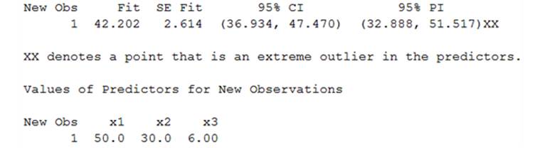
Figure-2
From Figure-2 it is clear that the confidence interval is
d.
To find: The prediction interval.
d.
Answer to Problem 21E
The prediction intervalis
Explanation of Solution
Given information: The data is shown below.
| 31.3 | 50 | 19 | 4.0 | 37.4 | 60 | 30 | 5.0 | 24.0 | 60 | 24 | 4.0 | 51.0 | 80 | 34 | 7.5 |
| 56.9 | 90 | 38 | 8.0 | 43.3 | 60 | 26 | 7.0 | 36.2 | 50 | 21 | 7.0 | 34.3 | 60 | 22 | 2.5 |
| 43.1 | 70 | 28 | 6.5 | 36.3 | 70 | 25 | 7.5 | 26.5 | 50 | 17 | 2.0 | 31.5 | 60 | 24 | 5.0 |
| 41.5 | 70 | 25 | 5.5 | 38.4 | 70 | 31 | 5.5 | 47.1 | 80 | 34 | 8.5 | 33.2 | 60 | 23 | 4.0 |
| 39.0 | 60 | 26 | 6.5 | 41.5 | 60 | 27 | 7.5 | 38.1 | 70 | 27 | 5.5 | 39.2 | 60 | 29 | 6.5 |
| 40.9 | 70 | 29 | 5.0 | 36.l | 60 | 23 | 6.0 | 33.5 | 60 | 24 | 2.5 | 46.7 | 70 | 27 | 7.5 |
| 35.9 | 60 | 23 | 5.5 | 38.5 | 60 | 23 | 6.0 | 43.6 | 70 | 27 | 10.0 | 30.4 | 70 | 32 | 4.0 |
| 43.5 | 70 | 28 | 5.5 | 42.4 | 60 | 24 | 9.0 | 41.0 | 80 | 32 | 6.5 | 43.2 | 60 | 25 | 5.5 |
| 47.9 | 80 | 34 | 6.5 | 46.5 | 70 | 31 | 5.5 | 50.2 | 50 | 26 | 9.0 | 30.6 | 60 | 26 | 3.5 |
| 33.8 | 70 | 26 | 4.5 | 43.1 | 80 | 32 | 6.0 | 34.4 | 50 | 22 | 4.0 | 43.3 | 70 | 28 | 7.5 |
| 41.1 | 70 | 26 | 8.0 | 50.8 | 60 | 26 | 10.0 | 47.9 | 80 | 34 | 6.5 | 32.4 | 60 | 22 | 5.5 |
| 38.7 | 70 | 26 | 8.0 | 44.2 | 70 | 28 | 4.5 | 46.2 | 50 | 21 | 10.0 | 35.5 | 60 | 22 | 4.5 |
Calculation:
From Figure-12 it is clear that the
e.
To find: The percentage of variation in variable
e.
Answer to Problem 21E
The percentage of variation in variable
Explanation of Solution
Given information: The data is shown below.
| 31.3 | 50 | 19 | 4.0 | 37.4 | 60 | 30 | 5.0 | 24.0 | 60 | 24 | 4.0 | 51.0 | 80 | 34 | 7.5 |
| 56.9 | 90 | 38 | 8.0 | 43.3 | 60 | 26 | 7.0 | 36.2 | 50 | 21 | 7.0 | 34.3 | 60 | 22 | 2.5 |
| 43.1 | 70 | 28 | 6.5 | 36.3 | 70 | 25 | 7.5 | 26.5 | 50 | 17 | 2.0 | 31.5 | 60 | 24 | 5.0 |
| 41.5 | 70 | 25 | 5.5 | 38.4 | 70 | 31 | 5.5 | 47.1 | 80 | 34 | 8.5 | 33.2 | 60 | 23 | 4.0 |
| 39.0 | 60 | 26 | 6.5 | 41.5 | 60 | 27 | 7.5 | 38.1 | 70 | 27 | 5.5 | 39.2 | 60 | 29 | 6.5 |
| 40.9 | 70 | 29 | 5.0 | 36.l | 60 | 23 | 6.0 | 33.5 | 60 | 24 | 2.5 | 46.7 | 70 | 27 | 7.5 |
| 35.9 | 60 | 23 | 5.5 | 38.5 | 60 | 23 | 6.0 | 43.6 | 70 | 27 | 10.0 | 30.4 | 70 | 32 | 4.0 |
| 43.5 | 70 | 28 | 5.5 | 42.4 | 60 | 24 | 9.0 | 41.0 | 80 | 32 | 6.5 | 43.2 | 60 | 25 | 5.5 |
| 47.9 | 80 | 34 | 6.5 | 46.5 | 70 | 31 | 5.5 | 50.2 | 50 | 26 | 9.0 | 30.6 | 60 | 26 | 3.5 |
| 33.8 | 70 | 26 | 4.5 | 43.1 | 80 | 32 | 6.0 | 34.4 | 50 | 22 | 4.0 | 43.3 | 70 | 28 | 7.5 |
| 41.1 | 70 | 26 | 8.0 | 50.8 | 60 | 26 | 10.0 | 47.9 | 80 | 34 | 6.5 | 32.4 | 60 | 22 | 5.5 |
| 38.7 | 70 | 26 | 8.0 | 44.2 | 70 | 28 | 4.5 | 46.2 | 50 | 21 | 10.0 | 35.5 | 60 | 22 | 4.5 |
Calculation:
From Figure-1 it is clear that the percentage of variation in variable
f.
To find:Whether the given model is useful for prediction.
f.
Answer to Problem 21E
The model is useful in prediction.
Explanation of Solution
Given information: The data is shown below.
| 31.3 | 50 | 19 | 4.0 | 37.4 | 60 | 30 | 5.0 | 24.0 | 60 | 24 | 4.0 | 51.0 | 80 | 34 | 7.5 |
| 56.9 | 90 | 38 | 8.0 | 43.3 | 60 | 26 | 7.0 | 36.2 | 50 | 21 | 7.0 | 34.3 | 60 | 22 | 2.5 |
| 43.1 | 70 | 28 | 6.5 | 36.3 | 70 | 25 | 7.5 | 26.5 | 50 | 17 | 2.0 | 31.5 | 60 | 24 | 5.0 |
| 41.5 | 70 | 25 | 5.5 | 38.4 | 70 | 31 | 5.5 | 47.1 | 80 | 34 | 8.5 | 33.2 | 60 | 23 | 4.0 |
| 39.0 | 60 | 26 | 6.5 | 41.5 | 60 | 27 | 7.5 | 38.1 | 70 | 27 | 5.5 | 39.2 | 60 | 29 | 6.5 |
| 40.9 | 70 | 29 | 5.0 | 36.l | 60 | 23 | 6.0 | 33.5 | 60 | 24 | 2.5 | 46.7 | 70 | 27 | 7.5 |
| 35.9 | 60 | 23 | 5.5 | 38.5 | 60 | 23 | 6.0 | 43.6 | 70 | 27 | 10.0 | 30.4 | 70 | 32 | 4.0 |
| 43.5 | 70 | 28 | 5.5 | 42.4 | 60 | 24 | 9.0 | 41.0 | 80 | 32 | 6.5 | 43.2 | 60 | 25 | 5.5 |
| 47.9 | 80 | 34 | 6.5 | 46.5 | 70 | 31 | 5.5 | 50.2 | 50 | 26 | 9.0 | 30.6 | 60 | 26 | 3.5 |
| 33.8 | 70 | 26 | 4.5 | 43.1 | 80 | 32 | 6.0 | 34.4 | 50 | 22 | 4.0 | 43.3 | 70 | 28 | 7.5 |
| 41.1 | 70 | 26 | 8.0 | 50.8 | 60 | 26 | 10.0 | 47.9 | 80 | 34 | 6.5 | 32.4 | 60 | 22 | 5.5 |
| 38.7 | 70 | 26 | 8.0 | 44.2 | 70 | 28 | 4.5 | 46.2 | 50 | 21 | 10.0 | 35.5 | 60 | 22 | 4.5 |
Calculation:
The null hypothesis is, the model is not useful for prediction and the alternative hypothesis is, the model is useful in prediction.
From Figure-1 it is clear that the p value is less than the level of significance of
Hence, the null hypothesis is rejected.
Thus, the model is useful in prediction.
g.
To explain:The test for the hypothesis
g.
Explanation of Solution
Given information: The data is shown below.
| 31.3 | 50 | 19 | 4.0 | 37.4 | 60 | 30 | 5.0 | 24.0 | 60 | 24 | 4.0 | 51.0 | 80 | 34 | 7.5 |
| 56.9 | 90 | 38 | 8.0 | 43.3 | 60 | 26 | 7.0 | 36.2 | 50 | 21 | 7.0 | 34.3 | 60 | 22 | 2.5 |
| 43.1 | 70 | 28 | 6.5 | 36.3 | 70 | 25 | 7.5 | 26.5 | 50 | 17 | 2.0 | 31.5 | 60 | 24 | 5.0 |
| 41.5 | 70 | 25 | 5.5 | 38.4 | 70 | 31 | 5.5 | 47.1 | 80 | 34 | 8.5 | 33.2 | 60 | 23 | 4.0 |
| 39.0 | 60 | 26 | 6.5 | 41.5 | 60 | 27 | 7.5 | 38.1 | 70 | 27 | 5.5 | 39.2 | 60 | 29 | 6.5 |
| 40.9 | 70 | 29 | 5.0 | 36.l | 60 | 23 | 6.0 | 33.5 | 60 | 24 | 2.5 | 46.7 | 70 | 27 | 7.5 |
| 35.9 | 60 | 23 | 5.5 | 38.5 | 60 | 23 | 6.0 | 43.6 | 70 | 27 | 10.0 | 30.4 | 70 | 32 | 4.0 |
| 43.5 | 70 | 28 | 5.5 | 42.4 | 60 | 24 | 9.0 | 41.0 | 80 | 32 | 6.5 | 43.2 | 60 | 25 | 5.5 |
| 47.9 | 80 | 34 | 6.5 | 46.5 | 70 | 31 | 5.5 | 50.2 | 50 | 26 | 9.0 | 30.6 | 60 | 26 | 3.5 |
| 33.8 | 70 | 26 | 4.5 | 43.1 | 80 | 32 | 6.0 | 34.4 | 50 | 22 | 4.0 | 43.3 | 70 | 28 | 7.5 |
| 41.1 | 70 | 26 | 8.0 | 50.8 | 60 | 26 | 10.0 | 47.9 | 80 | 34 | 6.5 | 32.4 | 60 | 22 | 5.5 |
| 38.7 | 70 | 26 | 8.0 | 44.2 | 70 | 28 | 4.5 | 46.2 | 50 | 21 | 10.0 | 35.5 | 60 | 22 | 4.5 |
The null hypothesis is, there is no relationship between
For the variable
From Figure-1 it is clear that the p value is
Hence, the null hypothesis is not rejected.
Thus, there is no linear relationship between
For the variable
From Figure-1 it is clear that the p value is
Hence, the null hypothesis is rejected.
Thus, there is alinear relationship between
For the variable
From Figure-1 it is clear that the p value is
Hence, the null hypothesis is rejected.
Thus, there is a linear relationship between
Want to see more full solutions like this?
Chapter 13 Solutions
Connect Hosted by ALEKS Access Card or Elementary Statistics


- The following relates to Problems 4 and 5. Christchurch, New Zealand experienced a major earthquake on February 22, 2011. It destroyed 100,000 homes. Data were collected on a sample of 300 damaged homes. These data are saved in the file called CIEG315 Homework 4 data.xlsx, which is available on Canvas under Files. A subset of the data is shown in the accompanying table. Two of the variables are qualitative in nature: Wall construction and roof construction. Two of the variables are quantitative: (1) Peak ground acceleration (PGA), a measure of the intensity of ground shaking that the home experienced in the earthquake (in units of acceleration of gravity, g); (2) Damage, which indicates the amount of damage experienced in the earthquake in New Zealand dollars; and (3) Building value, the pre-earthquake value of the home in New Zealand dollars. PGA (g) Damage (NZ$) Building Value (NZ$) Wall Construction Roof Construction Property ID 1 0.645 2 0.101 141,416 2,826 253,000 B 305,000 B T 3…arrow_forwardRose Par posted Apr 5, 2025 9:01 PM Subscribe To: Store Owner From: Rose Par, Manager Subject: Decision About Selling Custom Flower Bouquets Date: April 5, 2025 Our shop, which prides itself on selling handmade gifts and cultural items, has recently received inquiries from customers about the availability of fresh flower bouquets for special occasions. This has prompted me to consider whether we should introduce custom flower bouquets in our shop. We need to decide whether to start offering this new product. There are three options: provide a complete selection of custom bouquets for events like birthdays and anniversaries, start small with just a few ready-made flower arrangements, or do not add flowers. There are also three possible outcomes. First, we might see high demand, and the bouquets could sell quickly. Second, we might have medium demand, with a few sold each week. Third, there might be low demand, and the flowers may not sell well, possibly going to waste. These outcomes…arrow_forwardConsider the state space model X₁ = §Xt−1 + Wt, Yt = AX+Vt, where Xt Є R4 and Y E R². Suppose we know the covariance matrices for Wt and Vt. How many unknown parameters are there in the model?arrow_forward
- Business Discussarrow_forwardYou want to obtain a sample to estimate the proportion of a population that possess a particular genetic marker. Based on previous evidence, you believe approximately p∗=11% of the population have the genetic marker. You would like to be 90% confident that your estimate is within 0.5% of the true population proportion. How large of a sample size is required?n = (Wrong: 10,603) Do not round mid-calculation. However, you may use a critical value accurate to three decimal places.arrow_forward2. [20] Let {X1,..., Xn} be a random sample from Ber(p), where p = (0, 1). Consider two estimators of the parameter p: 1 p=X_and_p= n+2 (x+1). For each of p and p, find the bias and MSE.arrow_forward
- 1. [20] The joint PDF of RVs X and Y is given by xe-(z+y), r>0, y > 0, fx,y(x, y) = 0, otherwise. (a) Find P(0X≤1, 1arrow_forward4. [20] Let {X1,..., X} be a random sample from a continuous distribution with PDF f(x; 0) = { Axe 5 0, x > 0, otherwise. where > 0 is an unknown parameter. Let {x1,...,xn} be an observed sample. (a) Find the value of c in the PDF. (b) Find the likelihood function of 0. (c) Find the MLE, Ô, of 0. (d) Find the bias and MSE of 0.arrow_forward3. [20] Let {X1,..., Xn} be a random sample from a binomial distribution Bin(30, p), where p (0, 1) is unknown. Let {x1,...,xn} be an observed sample. (a) Find the likelihood function of p. (b) Find the MLE, p, of p. (c) Find the bias and MSE of p.arrow_forwardGiven the sample space: ΩΞ = {a,b,c,d,e,f} and events: {a,b,e,f} A = {a, b, c, d}, B = {c, d, e, f}, and C = {a, b, e, f} For parts a-c: determine the outcomes in each of the provided sets. Use proper set notation. a. (ACB) C (AN (BUC) C) U (AN (BUC)) AC UBC UCC b. C. d. If the outcomes in 2 are equally likely, calculate P(AN BNC).arrow_forwardSuppose a sample of O-rings was obtained and the wall thickness (in inches) of each was recorded. Use a normal probability plot to assess whether the sample data could have come from a population that is normally distributed. Click here to view the table of critical values for normal probability plots. Click here to view page 1 of the standard normal distribution table. Click here to view page 2 of the standard normal distribution table. 0.191 0.186 0.201 0.2005 0.203 0.210 0.234 0.248 0.260 0.273 0.281 0.290 0.305 0.310 0.308 0.311 Using the correlation coefficient of the normal probability plot, is it reasonable to conclude that the population is normally distributed? Select the correct choice below and fill in the answer boxes within your choice. (Round to three decimal places as needed.) ○ A. Yes. The correlation between the expected z-scores and the observed data, , exceeds the critical value, . Therefore, it is reasonable to conclude that the data come from a normal population. ○…arrow_forwardding question ypothesis at a=0.01 and at a = 37. Consider the following hypotheses: 20 Ho: μ=12 HA: μ12 Find the p-value for this hypothesis test based on the following sample information. a. x=11; s= 3.2; n = 36 b. x = 13; s=3.2; n = 36 C. c. d. x = 11; s= 2.8; n=36 x = 11; s= 2.8; n = 49arrow_forwardarrow_back_iosSEE MORE QUESTIONSarrow_forward_ios

 Glencoe Algebra 1, Student Edition, 9780079039897...AlgebraISBN:9780079039897Author:CarterPublisher:McGraw Hill
 Algebra: Structure And Method, Book 1AlgebraISBN:9780395977224Author:Richard G. Brown, Mary P. Dolciani, Robert H. Sorgenfrey, William L. ColePublisher:McDougal Littell
 Algebra & Trigonometry with Analytic GeometryAlgebraISBN:9781133382119Author:SwokowskiPublisher:Cengage