Concept explainers
Reminder Round all answers to two decimal places unless otherwise indicated.
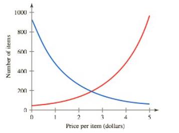
Equilibrium Price This is a continuation of Exorcise 5. The equilibrium price is the price where the supply and demand are the same. In Figure 1.31, the supply curve is in red and the demand curve is in blue. Use this graph to estimate the equilibrium price. How many items are supplied at the equilibrium price?

FIGURE
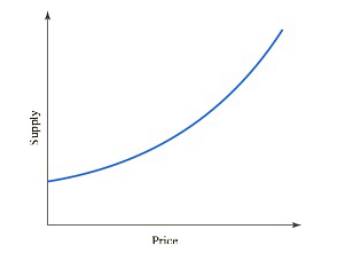
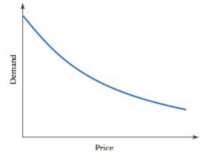
5. Supply and Demand Curves A supply curve is a graph that shows the quantity of a product that is made available by suppliers as a function of the price. Similarly, a demand curve is a graph that shows the quantity of a product that consumers are willing to purchase as a function of the price. Examples of supply and demand curves are shown in Figures
a. Explain in practical terms what the supply curve in Figure
b. Explain in practical terms what the demand curve in Figure 1.30 tells us.

FIGURE

FIGURE
Want to see the full answer?
Check out a sample textbook solution
Chapter 1 Solutions
Webassign Printed Access Card For Crauder/evans/noell's Functions And Change: A Modeling Approach To College Algebra, 6th Edition, Single-term
- I want to learn this topic l dont know anything about itarrow_forwardSolve the linear system of equations attached using Gaussian elimination (not Gauss-Jordan) and back subsitution. Remember that: A matrix is in row echelon form if Any row that consists only of zeros is at the bottom of the matrix. The first non-zero entry in each other row is 1. This entry is called aleading 1. The leading 1 of each row, after the first row, lies to the right of the leading 1 of the previous row.arrow_forwardPRIMERA EVALUACIÓN SUMATIVA 10. Determina la medida de los ángulos in- teriores coloreados en cada poligono. ⚫ Octágono regular A 11. Calcula es número de lados qu poligono regular, si la medida quiera de sus ángulos internos • a=156° A= (-2x+80 2 156 180- 360 0 = 24-360 360=24° • a = 162° 1620-180-360 6=18-360 360=19 2=360= 18 12. Calcula las medida ternos del cuadrilá B X+5 x+10 A X+X+ Sx+6 5x=3 x=30 0 лаб • Cuadrilátero 120° 110° • α = 166° 40' 200=180-360 0 = 26-360 360=20 ひ=360 20 18 J 60° ⚫a=169° 42' 51.43" 169.4143180-340 0 = 10.29 54-360 360 10.2857 2=360 10.2857 @Saarrow_forward
- Please help I'm a working mom trying to help my son last minute (6th grader)! Need help with the blank ones and check the ones he got with full calculation so we can use it to study! Especially the mixed number fractions cause I'm rusty. Thanks in advance!arrow_forward|| 38 5층-11- 6 4 7 2 6arrow_forwardMs.sally has 12 studentsMr Franklin has twice as many students as Ms. Sally.how many students does Mr Franklin have?arrow_forward
- explainwhat is means for a shape to be symmetricarrow_forwarde Grade Breakdown x Dashboard | Big Spring HX Dashboard | Big Spring H x Home | Lesson | Assessm cds.caolacourses.edisonlearning.com/lessons/assessmentplayer Co bigspringsd.org bookmarks Prodigy New Tab my video Brielynn... Algebra 2 Part 1-Exam-EDCP.MA003.A D Question 6 D ? 10 17°F Mostly sunny BSMS Home Significant Events in... Classes 25 26 27 28 29 30 31 32 33 34 35 36 37 38 39 40 Solve using row operations: x-3y= -4; 2x - y = 7 Use the paperclip button below to attach files. Student can enter max 2000 characters BISU DAIAAA X2 X2 T ② Type here Q Search e I ✓ Paragra Oarrow_forward1+3+5+7+ …+300 using gauss’s problemarrow_forward
 Functions and Change: A Modeling Approach to Coll...AlgebraISBN:9781337111348Author:Bruce Crauder, Benny Evans, Alan NoellPublisher:Cengage Learning
 Algebra and Trigonometry (MindTap Course List)AlgebraISBN:9781305071742Author:James Stewart, Lothar Redlin, Saleem WatsonPublisher:Cengage Learning
 Glencoe Algebra 1, Student Edition, 9780079039897...AlgebraISBN:9780079039897Author:CarterPublisher:McGraw Hill
 Algebra & Trigonometry with Analytic GeometryAlgebraISBN:9781133382119Author:SwokowskiPublisher:Cengage
 Trigonometry (MindTap Course List)TrigonometryISBN:9781337278461Author:Ron LarsonPublisher:Cengage Learning


