
Concept explainers
Videos
(a)
To find: The Inter
(a)
Answer to Problem 67E
Solution: The Inter
Explanation of Solution
Calculation: The Inter Quartile Range
Step 1: Enter the provided data in a Minitab worksheet.
Step 2: Go to Stat and select basic statistics.
Step 3: Then select Display
Step 4: Next click on Statistics tab and tick mark the option against interquartile range and click on OK twice to get the results.
From the Minitab output the Inter Quartile Range
Interpretation: The Inter Quartile Range
(b)
To find: The outliers using
(b)
Answer to Problem 67E
Solution: The value of outliers in the provided data is 428 of London. Any value above 236.5 or below –35.5 would be considered outliers as they are upper whisker and lower whisker, respectively.
Explanation of Solution
Calculation: To obtain the value of first and third quartile, follow the steps given below in Minitab,
Step 1: Enter the data in a Minitab worksheet.
Step 2: Go to Stat and select basic statistics.
Step 3: Then select Display Descriptive Statistics. Enter the name of the column containing the provided data in the variables textbox.
Step 4: Then click on Statistics tab and tick mark the option against first quartile and third quartile and click on OK twice.
The value of
The formula for upper whisker is,
where
The formula for lower whisker is,
where
Upper whisker of boxplot is found to be 236.5, so any values above 236.5 would be considered outliers and from data provided, value of 428 of London is outlier. There is no value below lower whisker.
Interpretation: Outliers refers to those data points that lie either above upper whisker and below lower whisker in boxplot. There was one outlier found in this data, and it is 428 of London.
(c)
To graph: A boxplot of the provided data and describe the distribution using it.
(c)
Explanation of Solution
Graph: Plot the boxplot in Minitab by performing the following steps,
Step 1: Enter the data into a Minitab worksheet.
Step 2: Go to ‘Graph’ and click on ‘Boxplot’.
Step 3: In the dialogue box that appears select ‘Simple’ and click OK.
Step 4: Next enter the name of the column containing the data in the filed marked as ‘Graph variables’ and click on OK.
The boxplot is obtained as shown below,
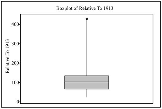
Interpretation: The boxplot is generally preferred to describe dataset having unsymmetrical distribution. The boxplot shows First quartile,
(d)
To graph: A modified boxplot and describes the distribution using it.
(d)
Explanation of Solution
Graph: Plot the modified boxplot in Minitab by performing the following steps,
Step 1: Enter the data into a Minitab worksheet.
Step 2: Go to ‘Graph’ and click on ‘Boxplot’.
Step 3: In the dialogue box that appears select ‘Simple’ and click OK.
Step 4: Next enter the name of the column containing the data in the filed marked as ‘Graph variables’ and click on OK.
The boxplot is obtained as shown below,
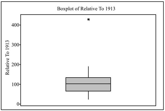
Interpretation: The modified boxplot is used to display data graphically when the distribution of data is unsymmetrical and skewed as it can clearly show outliers. In the modified boxplot it was found there is one data value which is upper outlier. This outlier is London. The modified boxplot does not display the outlier as a part of the whisker but marks the outlier away.
(e)
To graph: A stemplot of the provided data.
(e)
Explanation of Solution
Graph: Follow the steps given below to obtain the stemplot:
Step 1: Enter the data of sales in a Minitab worksheet.
Step 2: Go to Graph and select stem and leaves.
Step 3: Enter the name of the column containing the data in the Graph variables textbox and click OK.
The required stemplot is attached below,
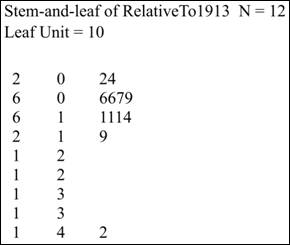
Interpretation: The stemplot of data is generally drawn when size of data is small and all the data values are positive. It shows all the data values on stemplot. In the stemplot shown above there is one outliers which is London whose data values is 428. Also the data does not seem to be symmetrically distributed.
(f)
To find: The comparison of Boxplot, Modified boxplot, and stemplot and mention advantages and disadvantages of each.
(f)
Answer to Problem 67E
Solution: In boxplot, data is displayed based on five-number summary, which included Minimum, Maximum, first quartile, third quartile, and Median and displaying the outlier as part of the whisker. In Modified boxplot also data is displayed based on five-number summary, but it displays the outliers such that they are not connected to the whiskers. In stemplot, data values are arranged in stem consisting of all digits except right most and leaves contain final digit. Advantage of boxplots is that it is suitable for unsymmetrical data while advantage of stemplot is that it shows all numerical value of data on graph itself. Disadvantage of Boxplot is that it is not suitable for unsymmetrical data while disadvantage of stemplot is that it is used only for positive numbers only and if the data size is small.
Explanation of Solution
The comparison of Boxplot, Modified boxplot, and stemplot is shown below:
Boxplot |
Modified Boxplot |
Stemplot |
|
Description |
It displays data based on |
It displays data based on five number summary including Minimum, Maximum, First quartile and Third Quartile and Median. The outliers are not displayed as part of the whiskers. |
In stemplot data values are arranged in stem consisting of all digits except right most digit and leaves contain final digit |
Advantages |
1. It displays five number summary graphically. 2. It is suitable for unsymmetrical data. |
1. It displays five number summary. 2. It is suitable for unsymmetrical data which is skewed. 3. It shows outliers clearly. |
1. It can display both symmetrical and unsymmetrical data graphically. 2. It can indicate outliers also 3. It displays all numerical values of data on stemplot. |
Disadvantages |
1. It is not suitable data set having symmetrical distribution. 2. It does not display outliers on graph. |
1. It is not suitable data set having symmetrical distribution. |
1. It is not suitable if data size is very large. 2. It is not used fornegative numbers. |
Want to see more full solutions like this?
Chapter 1 Solutions
Introduction to the Practice of Statistics


- The following ordered data list shows the data speeds for cell phones used by a telephone company at an airport: A. Calculate the Measures of Central Tendency using the table in point B. B. Are there differences in the measurements obtained in A and C? Why (give at least one justified reason)? 0.8 1.4 1.8 1.9 3.2 3.6 4.5 4.5 4.6 6.2 6.5 7.7 7.9 9.9 10.2 10.3 10.9 11.1 11.1 11.6 11.8 12.0 13.1 13.5 13.7 14.1 14.2 14.7 15.0 15.1 15.5 15.8 16.0 17.5 18.2 20.2 21.1 21.5 22.2 22.4 23.1 24.5 25.7 28.5 34.6 38.5 43.0 55.6 71.3 77.8arrow_forwardIn a company with 80 employees, 60 earn $10.00 per hour and 20 earn $13.00 per hour. a) Determine the average hourly wage. b) In part a), is the same answer obtained if the 60 employees have an average wage of $10.00 per hour? Prove your answer.arrow_forwardThe following ordered data list shows the data speeds for cell phones used by a telephone company at an airport: A. Calculate the Measures of Central Tendency from the ungrouped data list. B. Group the data in an appropriate frequency table. 0.8 1.4 1.8 1.9 3.2 3.6 4.5 4.5 4.6 6.2 6.5 7.7 7.9 9.9 10.2 10.3 10.9 11.1 11.1 11.6 11.8 12.0 13.1 13.5 13.7 14.1 14.2 14.7 15.0 15.1 15.5 15.8 16.0 17.5 18.2 20.2 21.1 21.5 22.2 22.4 23.1 24.5 25.7 28.5 34.6 38.5 43.0 55.6 71.3 77.8arrow_forward
- Businessarrow_forwardhttps://www.hawkeslearning.com/Statistics/dbs2/datasets.htmlarrow_forwardNC Current Students - North Ce X | NC Canvas Login Links - North ( X Final Exam Comprehensive x Cengage Learning x WASTAT - Final Exam - STAT → C webassign.net/web/Student/Assignment-Responses/submit?dep=36055360&tags=autosave#question3659890_9 Part (b) Draw a scatter plot of the ordered pairs. N Life Expectancy Life Expectancy 80 70 600 50 40 30 20 10 Year of 1950 1970 1990 2010 Birth O Life Expectancy Part (c) 800 70 60 50 40 30 20 10 1950 1970 1990 W ALT 林 $ # 4 R J7 Year of 2010 Birth F6 4+ 80 70 60 50 40 30 20 10 Year of 1950 1970 1990 2010 Birth Life Expectancy Ox 800 70 60 50 40 30 20 10 Year of 1950 1970 1990 2010 Birth hp P.B. KA & 7 80 % 5 H A B F10 711 N M K 744 PRT SC ALT CTRLarrow_forward
- Harvard University California Institute of Technology Massachusetts Institute of Technology Stanford University Princeton University University of Cambridge University of Oxford University of California, Berkeley Imperial College London Yale University University of California, Los Angeles University of Chicago Johns Hopkins University Cornell University ETH Zurich University of Michigan University of Toronto Columbia University University of Pennsylvania Carnegie Mellon University University of Hong Kong University College London University of Washington Duke University Northwestern University University of Tokyo Georgia Institute of Technology Pohang University of Science and Technology University of California, Santa Barbara University of British Columbia University of North Carolina at Chapel Hill University of California, San Diego University of Illinois at Urbana-Champaign National University of Singapore McGill…arrow_forwardName Harvard University California Institute of Technology Massachusetts Institute of Technology Stanford University Princeton University University of Cambridge University of Oxford University of California, Berkeley Imperial College London Yale University University of California, Los Angeles University of Chicago Johns Hopkins University Cornell University ETH Zurich University of Michigan University of Toronto Columbia University University of Pennsylvania Carnegie Mellon University University of Hong Kong University College London University of Washington Duke University Northwestern University University of Tokyo Georgia Institute of Technology Pohang University of Science and Technology University of California, Santa Barbara University of British Columbia University of North Carolina at Chapel Hill University of California, San Diego University of Illinois at Urbana-Champaign National University of Singapore…arrow_forwardA company found that the daily sales revenue of its flagship product follows a normal distribution with a mean of $4500 and a standard deviation of $450. The company defines a "high-sales day" that is, any day with sales exceeding $4800. please provide a step by step on how to get the answers in excel Q: What percentage of days can the company expect to have "high-sales days" or sales greater than $4800? Q: What is the sales revenue threshold for the bottom 10% of days? (please note that 10% refers to the probability/area under bell curve towards the lower tail of bell curve) Provide answers in the yellow cellsarrow_forward
- Find the critical value for a left-tailed test using the F distribution with a 0.025, degrees of freedom in the numerator=12, and degrees of freedom in the denominator = 50. A portion of the table of critical values of the F-distribution is provided. Click the icon to view the partial table of critical values of the F-distribution. What is the critical value? (Round to two decimal places as needed.)arrow_forwardA retail store manager claims that the average daily sales of the store are $1,500. You aim to test whether the actual average daily sales differ significantly from this claimed value. You can provide your answer by inserting a text box and the answer must include: Null hypothesis, Alternative hypothesis, Show answer (output table/summary table), and Conclusion based on the P value. Showing the calculation is a must. If calculation is missing,so please provide a step by step on the answers Numerical answers in the yellow cellsarrow_forwardShow all workarrow_forward
 MATLAB: An Introduction with ApplicationsStatisticsISBN:9781119256830Author:Amos GilatPublisher:John Wiley & Sons Inc
 Probability and Statistics for Engineering and th...StatisticsISBN:9781305251809Author:Jay L. DevorePublisher:Cengage Learning
 Statistics for The Behavioral Sciences (MindTap C...StatisticsISBN:9781305504912Author:Frederick J Gravetter, Larry B. WallnauPublisher:Cengage Learning
 Elementary Statistics: Picturing the World (7th E...StatisticsISBN:9780134683416Author:Ron Larson, Betsy FarberPublisher:PEARSON
 The Basic Practice of StatisticsStatisticsISBN:9781319042578Author:David S. Moore, William I. Notz, Michael A. FlignerPublisher:W. H. Freeman
 Introduction to the Practice of StatisticsStatisticsISBN:9781319013387Author:David S. Moore, George P. McCabe, Bruce A. CraigPublisher:W. H. Freeman