Concept explainers
Videos
a.
Construct a
a.
Answer to Problem 48CE
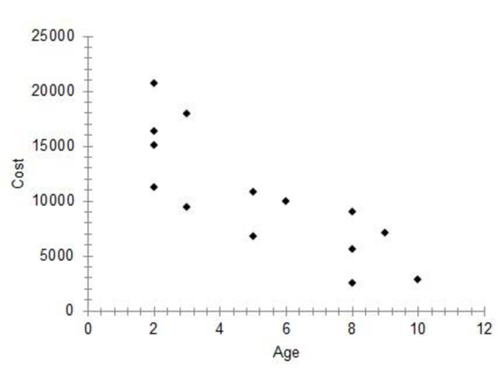
The scatter diagram of the data is as follows:
Explanation of Solution
It is given that ‘Estimated cost’ is the dependent variable.
Step-by-step procedure to obtain the scatterplot using the MegaStat software:
- In an EXCEL sheet enter the data values of x and y.
- Go to Add-Ins > MegaStat >
Correlation/Regression > Scatterplot. - Enter horizontal axis as $B$1:$B$15 and vertical axis as $A$1:$A$15.
- Click on OK.
From the scatterplot of the data, it indicates an inverse relationship.
b.
Find the
b.
Answer to Problem 48CE
The
Explanation of Solution
Step-by-step procedure to obtain the correlation coefficient using the MegaStat software:
- In an EXCEL sheet enter the data values of x and y.
- Go to Add-Ins > MegaStat > Correlation/Regression > Correlation matrix.
- Enter Input
Range as $A$1:$B$15. - Click on OK.
Output obtained using the MegaStat is given as follows:
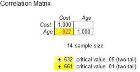
The correlation coefficient is –0.822. Since the correlation coefficient is negative and close to –1, there is a strong
c.
Interpret the slope of the regression equation.
c.
Explanation of Solution
The estimated regression equation is
The interpretation is that for each unit added to age, there is a decrease of $1,534 in cost.
d.
Estimate the cost of a five-year-old car.
d.
Answer to Problem 48CE
The estimated value of cost of a five-year-old car is $10,688.
Explanation of Solution
Substitute x as 5 in the regression equation.
Thus, the estimated value of cost of a five-year-old car is $10,688.
e.
Explain the given portion of the software output.
e.
Explanation of Solution
From the output p-value corresponding to the variable age is 0. That is, the p-value is less than any common level of significance. Thus, the variable age is significant.
f.
Test whether the slope is significant or not.
Interpret the result.
Check whether there is any significant relationship between the two variables.
f.
Answer to Problem 48CE
There is sufficient evidence to conclude that the slope of the regression line is different from zero at the 10% level of significance.
Explanation of Solution
It is given that the regression equation is
From the regression equation, the estimated slope of the regression line is
Let
The given test hypotheses are as follows:
Null hypothesis:
That is, the slope of the regression line is equal to zero.
Alternate hypothesis:
That is, the slope of the regression line is not equal to zero.
It is given that the level of significance is 0.10.
The standard error of
Test statistic:
The t-test statistic is as follows:
Where,
Thus, the following is obtained:
Here, the sample size is
Critical value:
Software procedure:
Step-by-step software procedure to obtain the critical value
- Open an EXCEL file.
- In cell A1, enter the formula “=T.INV(0.05,12)”.
Output obtained using the EXCEL is given as follows:
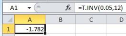
From the EXCEL output, the critical value is –1.782 (
Decision based on critical value:
Reject the null hypothesis, if
Conclusion:
The t-calculated value is 5.01 and the critical value is 1.782.
That is,
Thus, the null hypothesis is rejected.
Hence, there is sufficient evidence to conclude that the slope of the regression line is different from zero at the 10% level of significance.
Since the slope of the regression line is different from zero, there is a relationship between age and cost.
Want to see more full solutions like this?
Chapter 13 Solutions
EBK STATISTICAL TECHNIQUES IN BUSINESS


- Please help me answer the following questions from this problem.arrow_forwardPlease help me find the sample variance for this question.arrow_forwardCrumbs Cookies was interested in seeing if there was an association between cookie flavor and whether or not there was frosting. Given are the results of the last week's orders. Frosting No Frosting Total Sugar Cookie 50 Red Velvet 66 136 Chocolate Chip 58 Total 220 400 Which category has the greatest joint frequency? Chocolate chip cookies with frosting Sugar cookies with no frosting Chocolate chip cookies Cookies with frostingarrow_forward
- The table given shows the length, in feet, of dolphins at an aquarium. 7 15 10 18 18 15 9 22 Are there any outliers in the data? There is an outlier at 22 feet. There is an outlier at 7 feet. There are outliers at 7 and 22 feet. There are no outliers.arrow_forwardStart by summarizing the key events in a clear and persuasive manner on the article Endrikat, J., Guenther, T. W., & Titus, R. (2020). Consequences of Strategic Performance Measurement Systems: A Meta-Analytic Review. Journal of Management Accounting Research?arrow_forwardThe table below was compiled for a middle school from the 2003 English/Language Arts PACT exam. Grade 6 7 8 Below Basic 60 62 76 Basic 87 134 140 Proficient 87 102 100 Advanced 42 24 21 Partition the likelihood ratio test statistic into 6 independent 1 df components. What conclusions can you draw from these components?arrow_forward
- What is the value of the maximum likelihood estimate, θ, of θ based on these data? Justify your answer. What does the value of θ suggest about the value of θ for this biased die compared with the value of θ associated with a fair, unbiased, die?arrow_forwardShow that L′(θ) = Cθ394(1 −2θ)604(395 −2000θ).arrow_forwarda) Let X and Y be independent random variables both with the same mean µ=0. Define a new random variable W = aX +bY, where a and b are constants. (i) Obtain an expression for E(W).arrow_forward
- The table below shows the estimated effects for a logistic regression model with squamous cell esophageal cancer (Y = 1, yes; Y = 0, no) as the response. Smoking status (S) equals 1 for at least one pack per day and 0 otherwise, alcohol consumption (A) equals the average number of alcohoic drinks consumed per day, and race (R) equals 1 for blacks and 0 for whites. Variable Effect (β) P-value Intercept -7.00 <0.01 Alcohol use 0.10 0.03 Smoking 1.20 <0.01 Race 0.30 0.02 Race × smoking 0.20 0.04 Write-out the prediction equation (i.e., the logistic regression model) when R = 0 and again when R = 1. Find the fitted Y S conditional odds ratio in each case. Next, write-out the logistic regression model when S = 0 and again when S = 1. Find the fitted Y R conditional odds ratio in each case.arrow_forwardThe chi-squared goodness-of-fit test can be used to test if data comes from a specific continuous distribution by binning the data to make it categorical. Using the OpenIntro Statistics county_complete dataset, test the hypothesis that the persons_per_household 2019 values come from a normal distribution with mean and standard deviation equal to that variable's mean and standard deviation. Use signficance level a = 0.01. In your solution you should 1. Formulate the hypotheses 2. Fill in this table Range (-⁰⁰, 2.34] (2.34, 2.81] (2.81, 3.27] (3.27,00) Observed 802 Expected 854.2 The first row has been filled in. That should give you a hint for how to calculate the expected frequencies. Remember that the expected frequencies are calculated under the assumption that the null hypothesis is true. FYI, the bounderies for each range were obtained using JASP's drag-and-drop cut function with 8 levels. Then some of the groups were merged. 3. Check any conditions required by the chi-squared…arrow_forwardSuppose that you want to estimate the mean monthly gross income of all households in your local community. You decide to estimate this population parameter by calling 150 randomly selected residents and asking each individual to report the household’s monthly income. Assume that you use the local phone directory as the frame in selecting the households to be included in your sample. What are some possible sources of error that might arise in your effort to estimate the population mean?arrow_forward
 Glencoe Algebra 1, Student Edition, 9780079039897...AlgebraISBN:9780079039897Author:CarterPublisher:McGraw Hill
 Functions and Change: A Modeling Approach to Coll...AlgebraISBN:9781337111348Author:Bruce Crauder, Benny Evans, Alan NoellPublisher:Cengage Learning
 Algebra and Trigonometry (MindTap Course List)AlgebraISBN:9781305071742Author:James Stewart, Lothar Redlin, Saleem WatsonPublisher:Cengage Learning
 Algebra & Trigonometry with Analytic GeometryAlgebraISBN:9781133382119Author:SwokowskiPublisher:Cengage
 Holt Mcdougal Larson Pre-algebra: Student Edition...AlgebraISBN:9780547587776Author:HOLT MCDOUGALPublisher:HOLT MCDOUGAL