Videos
COMPENSATION FOR SALES PROFESSIONALS
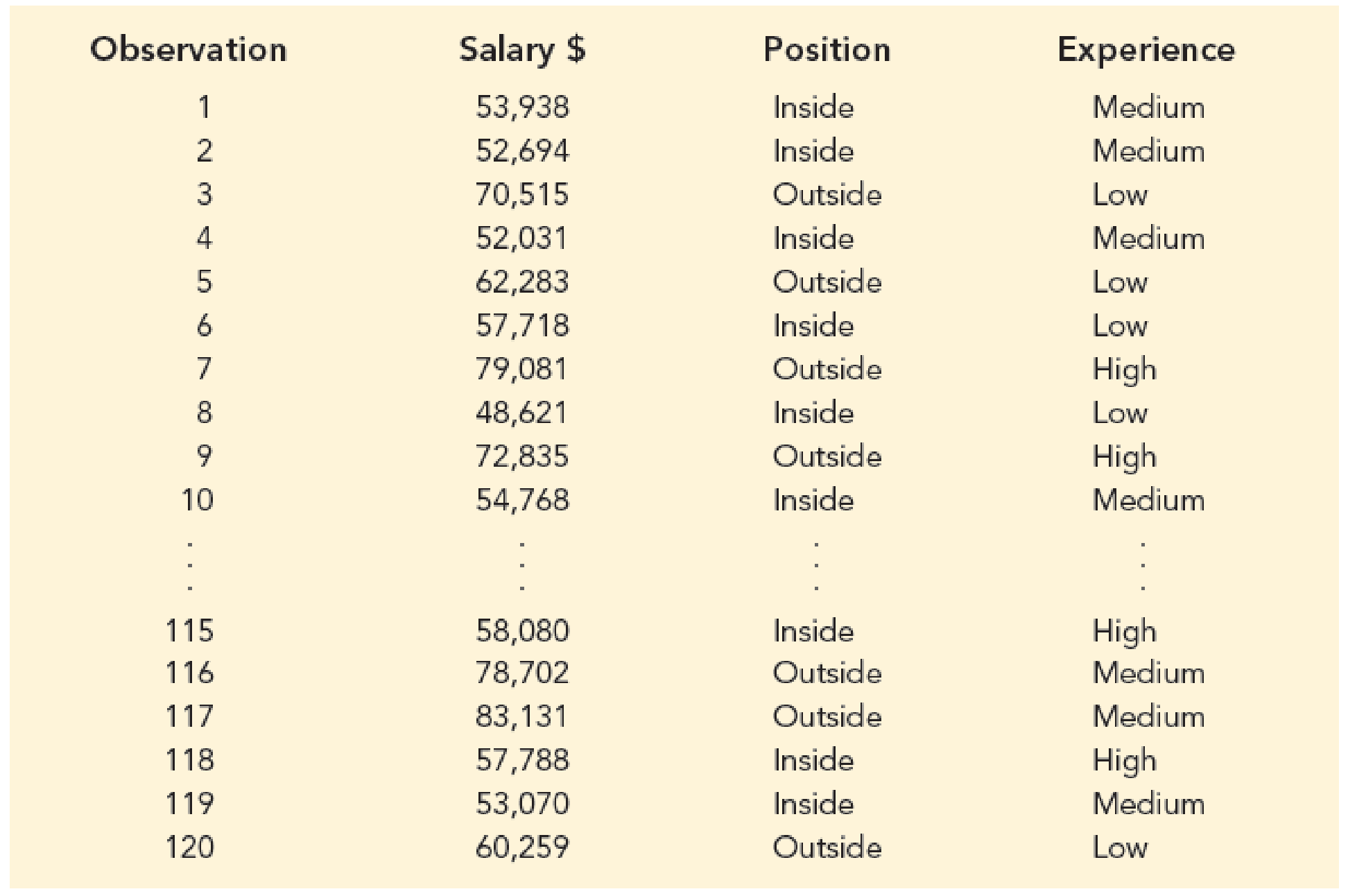
Suppose that a local chapter of sales professionals in the greater San Francisco area conducted a survey of its membership to study the relationship, if any, between the years of experience and salary for individuals employed in inside and outside sales positions. On the survey, respondents were asked to specify one of three levels of years of experience: low (1–10 years), medium (11–20 years), and high (21 or more years). A portion of the data obtained follow. The complete data set, consisting of 120 observations, is contained in the file named SalesSalary.
Managerial Report
- 1. Use
descriptive statistics to summarize the data. - 2. Develop a 95% confidence
interval estimate of themean annual salary for all salespersons, regardless of years of experience and type of position. - 3. Develop a 95% confidence interval estimate of the mean salary for inside salespersons.
- 4. Develop a 95% confidence interval estimate of the mean salary for outside salespersons.
- 5. Use analysis of variance to test for any significant differences due to position. Use a .05 level of significance, and for now, ignore the effect of years of experience.
- 6. Use analysis of variance to test for any significant differences due to years of experience. Use a .05 level of significance, and for now, ignore the effect of position.
- 7. At the .05 level of significance test for any significant differences due to position, years of experience, and interaction.
1.
Use descriptive statistics to summarize the data.
Explanation of Solution
Calculation:
The data represents the survey results obtained to study the relationship between the years of experience and salary for individuals employed in inside and outside sales positions. The respondents were asked to specify one of the three levels of years of experience: low, medium and high.
Descriptive statistics for the salary of individuals who employed inside sales position are shown below:
Software Procedure:
Step by step procedure to obtain the descriptive statistics using EXCEL:
- In a new EXCEL sheet enter 20 salaries of inside sales position persons at the three experience groups (low, high, medium).
- Go to Data > Data Analysis (in case it is not default, take the Analysis ToolPak from Excel Add Ins) > Descriptive statistics.
- Enter Input Range as $B$1:$D$21, select Columns in Grouped By, tick on Summary statistics.
- Click on OK.
Output using EXCEL is given as follows:
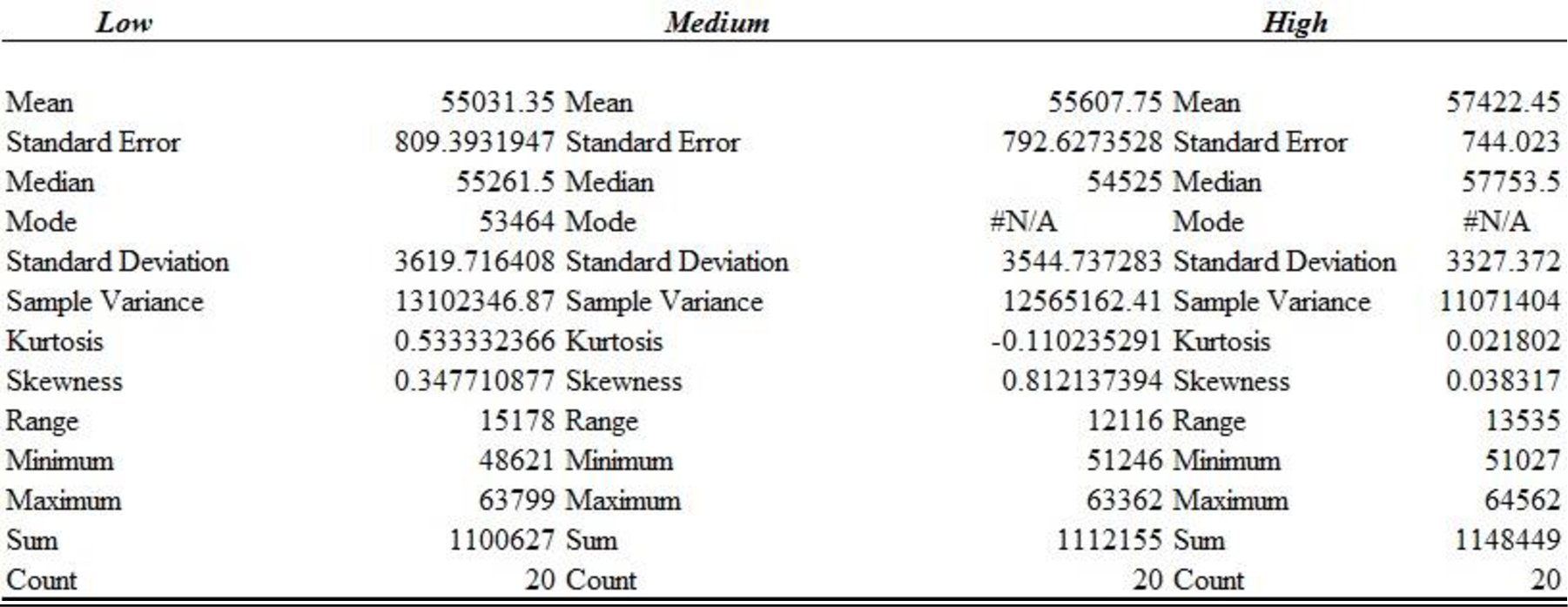
Thus, the descriptive statistics for the years of experience and salary for individuals employed in inside sales positions is obtained.
Descriptive statistics for the salary of individuals who employed outside sales position are shown below:
Software Procedure:
Step by step procedure to obtain the descriptive statistics using EXCEL:
- In a new EXCEL sheet enter 20 salaries of outside sales position persons at the three experience groups (low, high, medium).
- Go to Data > Data Analysis (in case it is not default, take the Analysis ToolPak from Excel Add Ins) > Descriptive statistics.
- Enter Input Range as $B$1:$D$21, select Columns in Grouped By, tick on Summary statistics.
- Click on OK.
Output using EXCEL is given as follows:
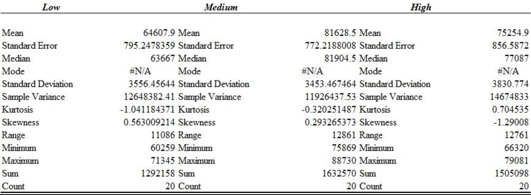
Thus, the descriptive statistics for the years of experience and salary for individuals employed in outside sales positions is obtained.
Descriptive statistics for the salary of individuals who employed inside and outside sales position are shown below:
Software Procedure:
Step by step procedure to obtain the descriptive statistics using EXCEL:
- In a new EXCEL sheet enter 40 salaries of inside and outside sales position persons at the three experience groups (low, high, medium)..
- Go to Data > Data Analysis (in case it is not default, take the Analysis ToolPak from Excel Add Ins) > Descriptive statistics.
- Enter Input Range as $B$1:$D$41, select Columns in Grouped By, tick on Summary statistics.
- Click on OK.
Output using EXCEL is given as follows:
Thus, the descriptive statistics for the years of experience and salary for individuals employed in inside and outside sales positions is obtained.
Descriptive statistics for the salary of individuals who employed in all sales position are shown below:
Software Procedure:
Step by step procedure to obtain the descriptive statistics using EXCEL:
- In a new EXCEL sheet enter all the 120 salaries in one column and label it as Total salary.
- Go to Data > Data Analysis (in case it is not default, take the Analysis ToolPak from Excel Add Ins) > Descriptive statistics.
- Enter Input Range as $B$1:$B$121, select Columns in Grouped By, tick on Summary statistics.
- Click on OK.
Output using EXCEL is given as follows:
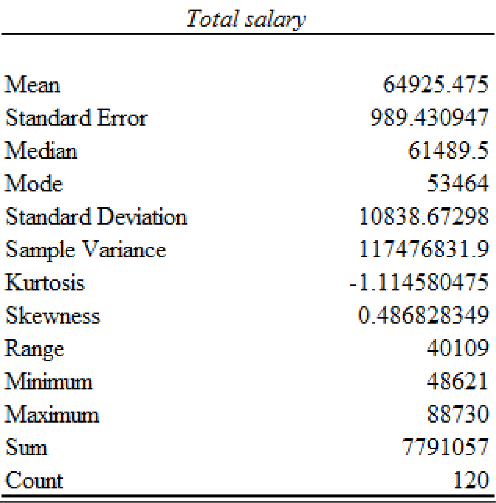
Thus, the descriptive statistics for the years of experience and salary for individuals employed in all sales positions is obtained.
The mean annual salary for sales persons regardless of years of experience and type of position is $64,925.48 and the standard deviation is $10,838.67. The mean salary for ‘Inside’ sales persons is $56,020.52 and the standard deviation is $3589.83. The mean salary for ‘Outside’ sales persons is $73,830.43 and the standard deviation is $7,922.96. The mean salary and standard deviation for ‘Outside’ sales persons is higher comparing with the mean salary for ‘Inside’ sales persons.
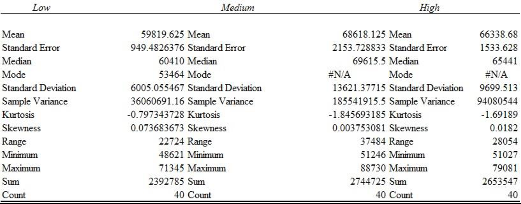
The mean salary for sales persons who have ‘Low’ years of experience is $59,819.63 and the standard deviation is $6,005.06.
The mean salary for sales persons who have ‘Medium’ years of experience is $68,618.13 and the standard deviation is $13,621.38.
The mean salary for sales persons who have ‘High’ years of experience is $66,338.68 and the standard deviation is $9,699.51.
The mean salary and standard deviation for sales persons who have ‘Medium’ years of experience is higher compared with the mean salary for sales persons who have ‘Low’ years of experience and ‘High’ years of experience.
2.
Develop a 95% confidence interval estimate of the mean annual salary for all sales persons regardless of years of experience and type of position.
Answer to Problem 2CP
The 95% confidence interval estimate of the mean annual salary for all sales persons regardless of years of experience and type of position is (62,966.41, 66,884.55).
Explanation of Solution
Calculation:
Here, 120 observations is considered as the sample and the population standard deviation is not known. Hence, t-test can be used for finding confidence intervals for testing population means.
The level of significance is 0.05.
Hence,
The 95% confidence interval for the mean annual salary for all sales persons regardless of years of experience and type of position is,
From part (a), substitute,
Critical value:
Software procedure:
Step-by-step procedure to obtain
- Open an EXCEL sheet.
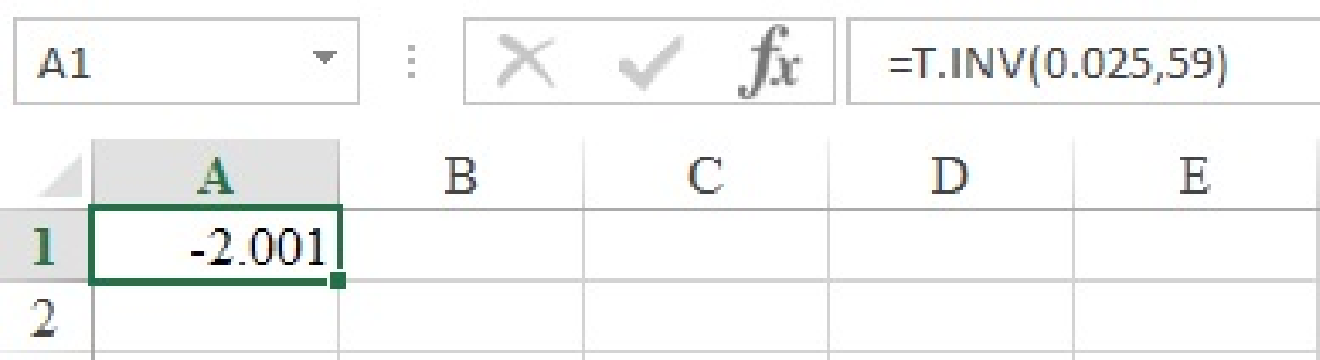
- Enter the formula in cell A1 as “=T.INV(0.025,119)”.
- Click on Enter.
Output using EXCEL software is given below:
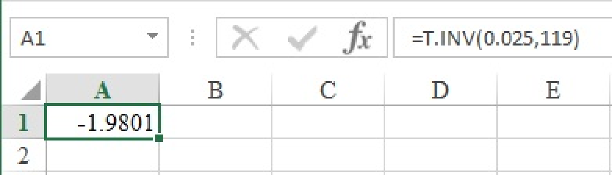
The value
The 95% confidence interval for the mean is,
Thus, the 95% confidence interval estimate of the mean annual salary for all sales persons regardless of years of experience and type of position is (62,966.41, 66,884.55).
3.
Develop a 95% confidence interval estimate of the mean salary for inside sales persons.
Answer to Problem 2CP
The 95% confidence interval estimate of the mean salary for inside sales persons is (56,947.87, 55,093.17).
Explanation of Solution
Calculation:
From part (a), the mean salary for the inside sales based on low, medium and high is given below:
The overall mean salary for inside sales person is provided below:
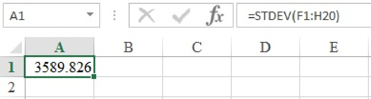
Standard deviation:
Software Procedure:
Step by step procedure to obtain the standard deviation using EXCEL:
- Open an EXCEL sheet.
- Enter the data.
- In a cell A1, enter the formula, “=STDEV(F1:H20)”.
- Click Enter.
Output using EXCEL software is given below:
substitute
Critical value:
Software procedure:
Step-by-step procedure to obtain
- Open an EXCEL sheet.
- Enter the formula in cell A1 as “=T.INV(0.025,119)”.
- Click on Enter.
Output using EXCEL software is given below:
The value
The 95% confidence interval for the mean is,
Thus, the 95% confidence interval estimate of the mean salary for inside sales persons is (56,947.87, 55,093.17).
4.
Develop a 95% confidence interval estimate of the mean salary for outside sales persons.
Answer to Problem 2CP
The 95% confidence interval estimate of the mean salary for outside sales persons is (75,877.15, 71,783.71).
Explanation of Solution
Calculation:
The 95% confidence interval for the mean salary for outside sales persons is,
The mean and standard deviation for salary of outside sales persons are
Here,
The 95% confidence interval for the mean is,
Thus, the 95% confidence interval estimate of the mean salary for inside sales persons is (56947.87, 55093.17).
5.
Check whether there are any significant differences due to position at
Answer to Problem 2CP
There is sufficient evidence to conclude that there is significant difference in the mean of positions at
Explanation of Solution
Calculation:
State the hypotheses:
Null hypothesis:
Alternative hypothesis:
The level of significance is 0.05.
One-way ANOVA:
Software procedure:
Step-by-step procedure to obtain the one-way Anova using the EXCEL:
- Open new EXCEL worksheet.
- Enter the data values in the cell.
- On Data tab in Analysis group, click Data Analysis.
- Select Anova: Single factor.
- Click Ok.
- Click in the Input Range box, select the range $A$1: $B$61.
- Select Labels and Enter Alpha as 0.05.
- Click in the Output range, select $G$1.
- Click OK.
Output using the EXCEL software is given below:
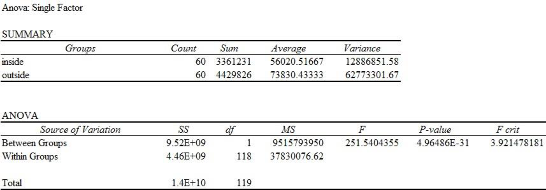
From the EXCEL output, the F-ratio is 251.54 and the p-value is 0.000.
Decision:
If
If
Conclusion:
Here, the p-value is less than the level of significance.
That is,
Therefore, the null hypothesis is rejected.
There is sufficient evidence to conclude that there is significant difference in the mean of positions at
6.
Check whether there are any significant differences due to years of experience at
Answer to Problem 2CP
There is sufficient evidence to conclude that there is significant difference in the mean of years of experience at
Explanation of Solution
Calculation:
State the hypotheses:
Null hypothesis:
Alternative hypothesis:
The level of significance is 0.05.
One-way ANOVA:
Software procedure:
Step-by-step procedure to obtain the one-way ANOVA using the EXCEL:
- Open new EXCEL worksheet.
- Enter the data values in the cell.
- On Data tab in Analysis group, click Data Analysis.
- Select Anova: Single factor.
- Click Ok.
- Click in the Input Range box, select the range $B$1: $D$41.
- Select Labels and Enter Alpha as 0.05.
- Click in the Output range, select $G$1.
- Click OK.
Output using the MINITAB software is given below:
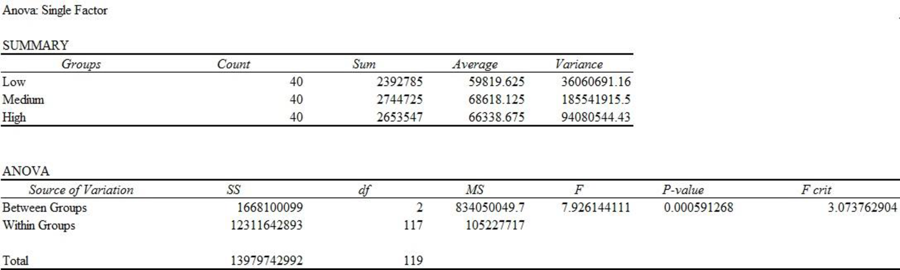
From the MINITAB output, the F-ratio is 7.93 and the p-value is 0.001.
Conclusion:
Here, the p-value is less than the level of significance.
That is,
Therefore, the null hypothesis is rejected.
There is sufficient evidence to conclude that there is significant difference in the mean of years of experience at
7.
Test for any significant differences due to position, years of experience and interaction at
Answer to Problem 2CP
The main effect of factor A (Position) is significant.
The main effect of factor B (Experience) is significant.
The interaction is significant.
Explanation of Solution
Calculation:
Factor A is Position (Inside, Outside). Factor B is Experience (Low, Medium, High).
The testing of hypotheses is as follows:
State the hypotheses:
Main effect of factor A:
Null hypothesis:
Alternative hypothesis:
Main effect of factor B:
Null hypothesis:
Alternative hypothesis:
Interaction:
Null hypothesis:
Alternative hypothesis:
Software procedure:
Step-by-step procedure to obtain the factorial experiment using the EXCEL:
- Open new EXCEL worksheet.
- Enter the data values in the cell.
- On Data tab in Analysis group, click Data Analysis.
- Select Anova: Two-Factor With Replication.
- Click Ok.
- Click in the Input Range box, select the range $A$1: $E$11.
- Click in the Rows per sample, Enter 2.
- Select Labels and Enter Alpha as 0.05.
- Click in the Output range, select $G$1.
- Click OK.
Output obtained by EXCEL procedure is as follows:
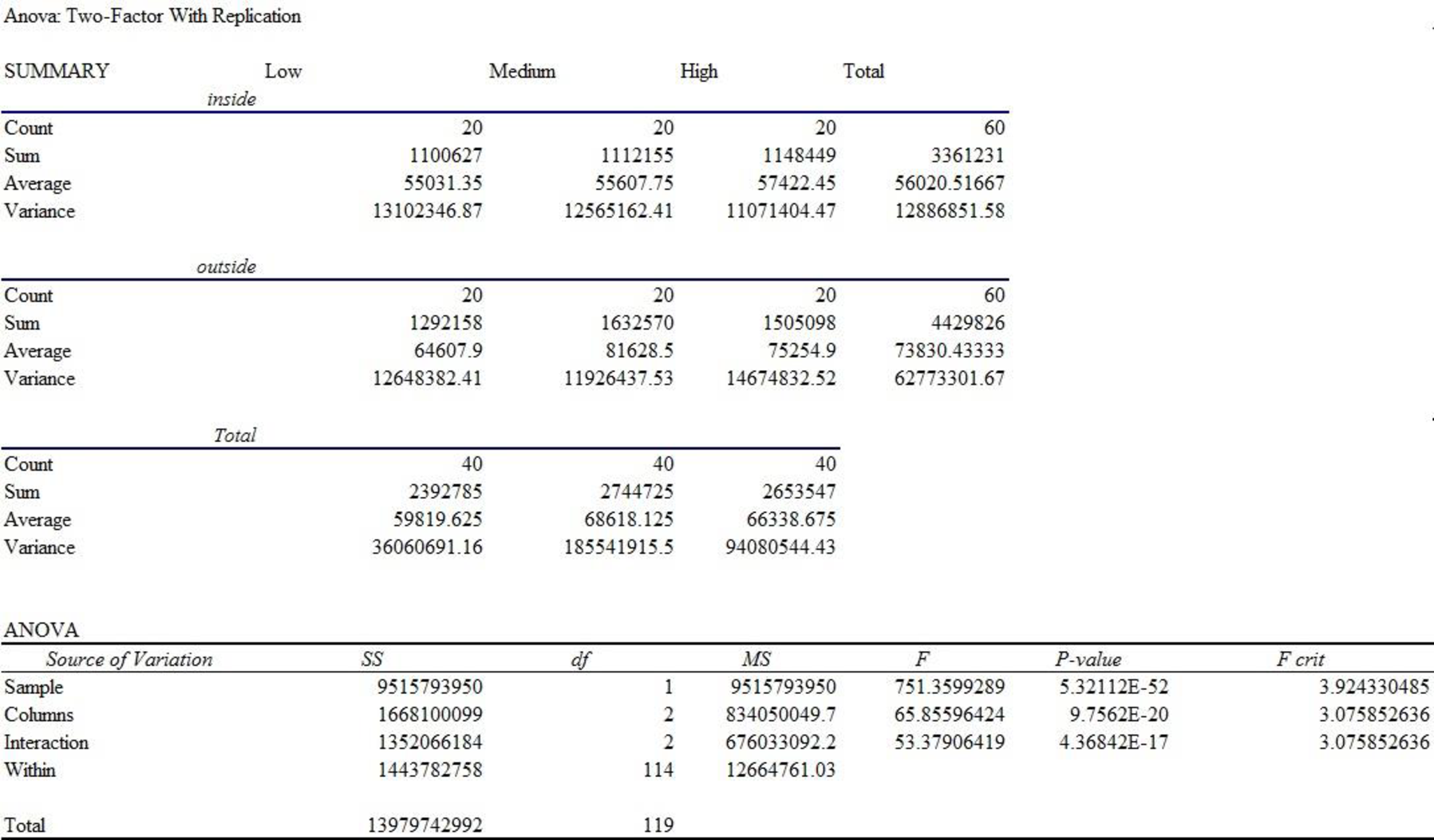
For Factor A (Position), the F-test statistic is 751.36 and the p-value is 0.000.
For Factor B (Experience), the F-test statistic is 65.86 and the p-value is 0.000.
For interaction, the F-test statistic is 53.38 and the p-value is 0.000.
Decision:
If
If
Conclusion:
Factor A:
Here, the p-value is less than the level of significance.
That is,
Therefore, the null hypothesis is rejected.
That is, the main effect of factor A (Position) is significant.
Factor B:
Here, the p-value is less than the level of significance.
That is,
Therefore, the null hypothesis is rejected.
That is, the main effect of factor B (Experience) is significant.
Interaction:
Here, the p-value is less than the level of significance.
That is,
Therefore, the null hypothesis is rejected.
Thus, the interaction is significant.
Want to see more full solutions like this?
Chapter 13 Solutions
Modern Business Statistics with Microsoft Excel (MindTap Course List)


- Suppose a random sample of 459 married couples found that 307 had two or more personality preferences in common. In another random sample of 471 married couples, it was found that only 31 had no preferences in common. Let p1 be the population proportion of all married couples who have two or more personality preferences in common. Let p2 be the population proportion of all married couples who have no personality preferences in common. Find a95% confidence interval for . Round your answer to three decimal places.arrow_forwardA history teacher interviewed a random sample of 80 students about their preferences in learning activities outside of school and whether they are considering watching a historical movie at the cinema. 69 answered that they would like to go to the cinema. Let p represent the proportion of students who want to watch a historical movie. Determine the maximal margin of error. Use α = 0.05. Round your answer to three decimal places. arrow_forwardA random sample of medical files is used to estimate the proportion p of all people who have blood type B. If you have no preliminary estimate for p, how many medical files should you include in a random sample in order to be 99% sure that the point estimate will be within a distance of 0.07 from p? Round your answer to the next higher whole number.arrow_forward
- A clinical study is designed to assess the average length of hospital stay of patients who underwent surgery. A preliminary study of a random sample of 70 surgery patients’ records showed that the standard deviation of the lengths of stay of all surgery patients is 7.5 days. How large should a sample to estimate the desired mean to within 1 day at 95% confidence? Round your answer to the whole number.arrow_forwardA clinical study is designed to assess the average length of hospital stay of patients who underwent surgery. A preliminary study of a random sample of 70 surgery patients’ records showed that the standard deviation of the lengths of stay of all surgery patients is 7.5 days. How large should a sample to estimate the desired mean to within 1 day at 95% confidence? Round your answer to the whole number.arrow_forwardIn the experiment a sample of subjects is drawn of people who have an elbow surgery. Each of the people included in the sample was interviewed about their health status and measurements were taken before and after surgery. Are the measurements before and after the operation independent or dependent samples?arrow_forward
- iid 1. The CLT provides an approximate sampling distribution for the arithmetic average Ỹ of a random sample Y₁, . . ., Yn f(y). The parameters of the approximate sampling distribution depend on the mean and variance of the underlying random variables (i.e., the population mean and variance). The approximation can be written to emphasize this, using the expec- tation and variance of one of the random variables in the sample instead of the parameters μ, 02: YNEY, · (1 (EY,, varyi n For the following population distributions f, write the approximate distribution of the sample mean. (a) Exponential with rate ẞ: f(y) = ß exp{−ßy} 1 (b) Chi-square with degrees of freedom: f(y) = ( 4 ) 2 y = exp { — ½/ } г( (c) Poisson with rate λ: P(Y = y) = exp(-\} > y! y²arrow_forward2. Let Y₁,……., Y be a random sample with common mean μ and common variance σ². Use the CLT to write an expression approximating the CDF P(Ỹ ≤ x) in terms of µ, σ² and n, and the standard normal CDF Fz(·).arrow_forwardmatharrow_forward
- Compute the median of the following data. 32, 41, 36, 42, 29, 30, 40, 22, 25, 37arrow_forwardTask Description: Read the following case study and answer the questions that follow. Ella is a 9-year-old third-grade student in an inclusive classroom. She has been diagnosed with Emotional and Behavioural Disorder (EBD). She has been struggling academically and socially due to challenges related to self-regulation, impulsivity, and emotional outbursts. Ella's behaviour includes frequent tantrums, defiance toward authority figures, and difficulty forming positive relationships with peers. Despite her challenges, Ella shows an interest in art and creative activities and demonstrates strong verbal skills when calm. Describe 2 strategies that could be implemented that could help Ella regulate her emotions in class (4 marks) Explain 2 strategies that could improve Ella’s social skills (4 marks) Identify 2 accommodations that could be implemented to support Ella academic progress and provide a rationale for your recommendation.(6 marks) Provide a detailed explanation of 2 ways…arrow_forwardQuestion 2: When John started his first job, his first end-of-year salary was $82,500. In the following years, he received salary raises as shown in the following table. Fill the Table: Fill the following table showing his end-of-year salary for each year. I have already provided the end-of-year salaries for the first three years. Calculate the end-of-year salaries for the remaining years using Excel. (If you Excel answer for the top 3 cells is not the same as the one in the following table, your formula / approach is incorrect) (2 points) Geometric Mean of Salary Raises: Calculate the geometric mean of the salary raises using the percentage figures provided in the second column named “% Raise”. (The geometric mean for this calculation should be nearly identical to the arithmetic mean. If your answer deviates significantly from the mean, it's likely incorrect. 2 points) Starting salary % Raise Raise Salary after raise 75000 10% 7500 82500 82500 4% 3300…arrow_forward
 Functions and Change: A Modeling Approach to Coll...AlgebraISBN:9781337111348Author:Bruce Crauder, Benny Evans, Alan NoellPublisher:Cengage Learning
 Big Ideas Math A Bridge To Success Algebra 1: Stu...AlgebraISBN:9781680331141Author:HOUGHTON MIFFLIN HARCOURTPublisher:Houghton Mifflin Harcourt
 Glencoe Algebra 1, Student Edition, 9780079039897...AlgebraISBN:9780079039897Author:CarterPublisher:McGraw Hill
 Linear Algebra: A Modern IntroductionAlgebraISBN:9781285463247Author:David PoolePublisher:Cengage Learning