Subpart (a):
Marginal revenue.
Subpart (a):
Explanation of Solution
In case A, part (I):
Marginal revenue equation can be derived as follows:
Marginal revenue equation is 50-2Q.
When the quantity is 0 units, the marginal revenue can be calculated by substituting the respective values in the marginal revenue equation.
Marginal revenue is 50 at the point where the quantity is 0 units.
When the quantity is 25 units, the marginal revenue can be calculated by substituting the respective values in the marginal revenue equation.
Marginal revenue is 0 at the point where the quantity is 50 units.
Figure 1 illustrates the marginal revenue curve for 50-2Q.
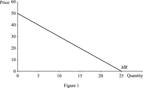
In Figure 1, the vertical axis measures price and the horizontal axis measures quantity; when the quantity is zero, the price would be 50. At price zero, the quantity demanded is 25; thus, this joins the two points the marginal revenue curve gets.
In case A, part (II):
The profit-maximizing output can be calculated by equating the marginal revenue to the marginal cost. This can be done as follows:
Profit-maximizing output is 20 units.
In case A, part (III):
Substitute the profit-maximizing output in the
Profit-maximizing price is $30.
In case A, part (IV):
Total revenue can be obtained by multiplying the profit-maximizing price with the profit-maximizing quantity. This can be done as follows:
Total revenue is $600.
Total cost can be calculated as follows:
Total cost is $300.
In case A, part (V):
Profit can be calculated as follows:
Profit is $300.
In case B, part (I):
Marginal revenue equation can be derived as follows:
Marginal revenue equation is 100-4Q.
When quantity is 0 units, the marginal revenue can be calculated by substituting the respective values in the marginal revenue equation.
Marginal revenue is 100 at the point where the quantity is 0 units.
When quantity is 25 units, the marginal revenue can be calculated by substituting the respective values in the marginal revenue equation.
Marginal revenue is 0 at the point where the quantity is 50 units.
Figure 2 illustrates the marginal revenue curve for 100-4Q.
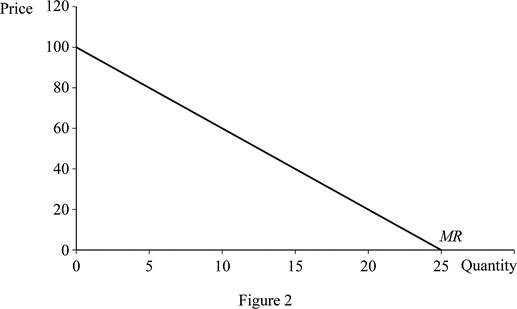
In Figure 2, the vertical axis measures price and the horizontal axis measures quantity. When the quantity is zero, the price would be 100, and at price zero, the quantity demanded is 25. Thus, joining the two points can help obtain the marginal revenue curve.
In case B, part (II):
Profit-maximizing output can be calculated by equating the marginal revenue to the marginal cost. This can be done as follows:
Profit-maximizing output is 22.5 units.
In case B, part (III):
Substitute the profit-maximizing output in the demand equation to calculate the profit maximizing price.
Profit-maximizing price is $55.
In case B, part (IV):
Total revenue can be obtained by multiplying the profit-maximizing price with profit-maximizing quantity. This can be done as follows:
Total revenue is $1,237.5.
Total cost can be calculated as follows:
Total cost is $325.
In case B, part (V):
Profit can be calculated as follows:
Profit is $912.5.
In case C, part (I):
Marginal revenue equation can be derived as follows:
Marginal revenue equation is 100-4Q.
When the quantity is 0 units, the marginal revenue can be calculated by substituting the respective values in the marginal revenue equation.
Marginal revenue is 100 at the point where the quantity is 0 units.
When the quantity is 25 units, the marginal revenue can be calculated by substituting the respective values in the marginal revenue equation.
Marginal revenue is 0 at the point where the quantity is 50 units.
Figure 3 illustrates the marginal revenue curve for100-4Q.
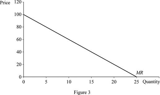
In Figure 3, the vertical axis measures price and the horizontal axis measures quantity. When the quantity is zero, the price would be 100, and at price zero, the quantity demanded is 25. Thus, joining the two points can help obtain the marginal revenue curve.
In case C, part (II):
Profit-maximizing output can be calculated by equating marginal revenue to the marginal cost. This can be done as follows:
Profit-maximizing output is 20 units.
In case C, part (III):
Substitute the profit-maximizing output in demand equation to calculate the profit-maximizing price.
Profit-maximizing price is $60.
In case C, part (IV):
Total revenue can be obtained by multiplying the profit-maximizing price with profit-maximizing quantity. This can be done as follows:
Total revenue is $1,200.
Total cost can be calculated as follows:
Total cost is $500.
In case C, part (V):
Profit can be calculated as follows:
Profit is $700.
Concept introduction:
Marginal revenue: The change in total revenue from selling an additional unit is known as marginal revenue.
Mark-up: Mark-up refers to the amount that is added by the seller to the cost of the goods to determine the selling price.
Sub part (b):
Marginal revenue.
Sub part (b):
Explanation of Solution
The markup refers to the amount that is added by the seller to the cost of the goods to determine the selling price. For calculating the percentage markup, the following equation can be used:
Case A:
Using equation (1), the percentage mark-up in case A can be calculated as follows:
The percentage mark-up in price $20 is 200%.
Case B:
To calculate the percentage mark-up in case B, substitute the values in equation (1).
The percentage mark-up in price $45 is 450%.
Case C:
To calculate the percentage mark-up in case C, substitute the values in equation (1).
The percentage mark-up in price $40 is 200%.
Concept introduction:
Marginal revenue: The change in total revenue from selling an additional unit is known as marginal revenue.
Mark-up: Mark-up refers to the amount that is added by the seller to the cost of the goods to determine the selling price.
Sub part (c):
Marginal revenue.
Sub part (c):
Explanation of Solution
If
Want to see more full solutions like this?
Chapter 13 Solutions
EBK MODERN PRINCIPLES OF ECONOMICS

- Sue is a sole proprietor of her own sewing business. Revenues are $150,000 per year and raw material (cloth, thread) costs are $130,000 per year. Sue pays herself a salary of $60,000 per year but gave up a job with a salary of $80,000 to run the business. ○ A. Her accounting profits are $0. Her economic profits are - $60,000. ○ B. Her accounting profits are $0. Her economic profits are - $40,000. ○ C. Her accounting profits are - $40,000. Her economic profits are - $60,000. ○ D. Her accounting profits are - $60,000. Her economic profits are -$40,000.arrow_forwardSelect a number that describes the type of firm organization indicated. Descriptions of Firm Organizations: 1. has one owner-manager who is personally responsible for all aspects of the business, including its debts 2. one type of partner takes part in managing the firm and is personally liable for the firm's actions and debts, and the other type of partner takes no part in the management of the firm and risks only the money that they have invested 3. owners are not personally responsible for anything that is done in the name of the firm 4. owned by the government but is usually under the direction of a more or less independent, state-appointed board 5. established with the explicit objective of providing goods or services but only in a manner that just covers its costs 6. has two or more joint owners, each of whom is personally responsible for all of the partnership's debts Type of Firm Organization a. limited partnership b. single proprietorship c. corporation Correct Numberarrow_forwardThe table below provides the total revenues and costs for a small landscaping company in a recent year. Total Revenues ($) 250,000 Total Costs ($) - wages and salaries 100,000 -risk-free return of 2% on owner's capital of $25,000 500 -interest on bank loan 1,000 - cost of supplies 27,000 - depreciation of capital equipment 8,000 - additional wages the owner could have earned in next best alternative 30,000 -risk premium of 4% on owner's capital of $25,000 1,000 The economic profits for this firm are ○ A. $83,000. B. $82,500. OC. $114,000. OD. $83,500. ○ E. $112,500.arrow_forward
- Output TFC ($) TVC ($) TC ($) (Q) 2 100 104 204 3 100 203 303 4 100 300 400 5 100 405 505 6 100 512 612 7 100 621 721 Given the information about short-run costs in the table above, we can conclude that the firm will minimize the average total cost of production when Q = (Round your response to the nearest whole number.)arrow_forwardThe following data show the total output for a firm when specified amounts of labour are combined with a fixed amount of capital. Assume that the wage per unit of labour is $20 and the cost of the capital is $100. Labour per unit of time 0 1 Total Output 0 25 T 2 3 4 5 75 137 212 267 The marginal product of labour is at its maximum when the firm changes the amount of labour hired from ○ A. 0 to 1 unit. ○ B. 3 to 4 units. OC. 2 to 3 units. OD. 1 to 2 units. ○ E. 4 to 5 units.arrow_forwardThe table below provides the annual revenues and costs for a family-owned firm producing catered meals. Total Revenues ($) 600,000 Total Costs ($) - wages and salaries 250,000 -risk-free return of 7% on owners' capital of $300,000 21,000 - rent 101,000 - depreciation of capital equipment 22,000 -risk premium of 9% on owners' capital of $300,000 27,000 - intermediate inputs 146,000 -forgone wages of owners in alternative employment -interest on bank loan 70,000 11,000 The implicit costs for this family-owned firm are ○ A. $70,000. OB. $97,000. OC. $589,000. OD. $118,000. ○ E. $48,000.arrow_forward
- Suppose a production function for a firm takes the following algebraic form: Q= 2KL - (0.3)L², where Q is the output of sweaters per day. Now suppose the firm is operating with 10 units of capital (K = 10) and 6 units of labour (L = 6). What is the output of sweaters? A. 64 sweaters per day OB. 49 sweaters per day OC. 109 sweaters per day OD. 72 sweaters per day OE. 118 sweaters per dayarrow_forward3. Consider a course allocation problem with strict and non-responsive preferences. Isthere a mechanism that is efficient and strategy-proof? If so, state the mechanismand show that it satisfies efficiency and strategyproofness. {hint serial dictatorship and show using example}4. Consider a course allocation problem with responsive preferences and at least 3students. Is there a mechanism that is efficient and strategy-proof that is not theSerial Dictatorship? If so, state the mechanism and show that it satisfies efficiencyand strategyproofness.5. Suggest a mechanism for allocating students to courses in a situation where preferences are non-responsive, and study its properties (efficiency and strategyproofness). Please be creativearrow_forward3. Consider a course allocation problem with strict and non-responsive preferences. Isthere a mechanism that is efficient and strategy-proof? If so, state the mechanismand show that it satisfies efficiency and strategyproofness. {hint serial dictatorship}4. Consider a course allocation problem with responsive preferences and at least 3students. Is there a mechanism that is efficient and strategy-proof that is not theSerial Dictatorship? If so, state the mechanism and show that it satisfies efficiencyand strategyproofness.5. Suggest a mechanism for allocating students to courses in a situation where preferences are non-responsive, and study its properties (efficiency and strategyproofness). Please be creativearrow_forward

 Principles of Economics (12th Edition)EconomicsISBN:9780134078779Author:Karl E. Case, Ray C. Fair, Sharon E. OsterPublisher:PEARSON
 Engineering Economy (17th Edition)EconomicsISBN:9780134870069Author:William G. Sullivan, Elin M. Wicks, C. Patrick KoellingPublisher:PEARSON
 Principles of Economics (MindTap Course List)EconomicsISBN:9781305585126Author:N. Gregory MankiwPublisher:Cengage Learning
 Managerial Economics: A Problem Solving ApproachEconomicsISBN:9781337106665Author:Luke M. Froeb, Brian T. McCann, Michael R. Ward, Mike ShorPublisher:Cengage Learning
 Managerial Economics & Business Strategy (Mcgraw-...EconomicsISBN:9781259290619Author:Michael Baye, Jeff PrincePublisher:McGraw-Hill Education