Concept explainers
Videos
a.
Check whether a linear model is appropriate for the data using the
a.
Answer to Problem 48E
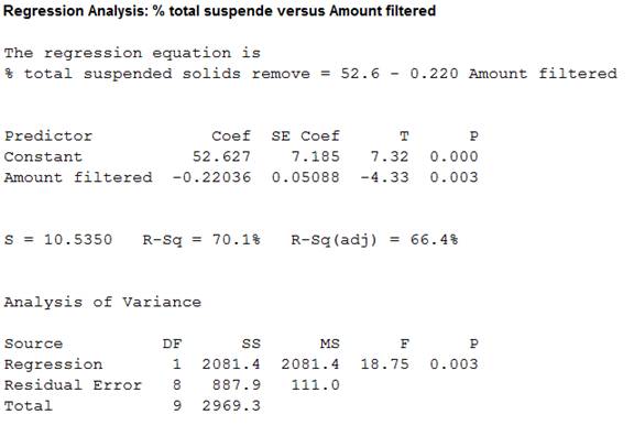
Output using MINITAB software is given below:
Yes, a simple linear model is appropriate for the data.
Explanation of Solution
Given info:
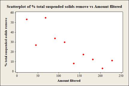
The data represents the values of the variables % total suspended solids removed
Justification:
Software Procedure:
Step by step procedure to obtain scatterplot using MINITAB software is given as,
- Choose Graph > Scatter plot.
- Choose Simple, and then click OK.
- Under Y variables, enter a column of % Total suspended solids removed.
- Under X variables, enter a column of Amount filtered.
- Click Ok.
Observation:
From the scatterplot it is clear that, as the values of amount filtered increases the values of % total suspended solids removed decreases linearly. Thus, there is a negative association between the variables amount filtered and % total suspended solids removed.
Appropriateness of regression linear model:
The conditions for a scatterplot that is well fitted for the data are,
- Straight Enough Condition: The relationship between y and x straight enough to proceed with a linear regression model.
- Outlier Condition: No outlier must be there which influences the fit of the least square line.
- Thickness Condition: The spread of the data around the generally straight relationship seem to be consistent for all values of x.
The scatterplot shows a fair enough linear relationship between the variables amount filtered and % total suspended solids removed. The spread of the data seem to roughly consistent.
Moreover, the scatterplot does not show any outliers.
Therefore, all the three conditions of appropriateness of simple linear model are satisfied.
Thus, a linear model is appropriate for the data.
b.
Find the regression line for the variables % total suspended solids removed
b.
Answer to Problem 48E
The regression line for the variables % total suspended solids removed
Explanation of Solution
Calculation:
Linear regression model:
A linear regression model is given as
A linear regression model is given as
In the given problem the % of total suspended solids remove is the response variable y and the amount filtered is the predictor variable x
Regression:
Software procedure:
Step by step procedure to obtain regression equation using MINITAB software is given as,
- Choose Stat > Regression > Fit Regression Line.
- In Response (Y), enter the column of Removal efficiency.
- In Predictor (X), enter the column of Inlet temperature.
- Click OK.
The output using MINITAB software is given as,
Thus, the regression line for the variables % total suspended solids removed
Interpretation:
The slope estimate implies a decrease in % total suspended solids removed by 22.0% for every 1,000 liters increase in amount filtered. It can also be said that, for every 1% increase in amount filtered the % total suspended solids removed decreases 22%.
c.
Find the proportion of observed variation in % total suspended solids removed that can be explained by amount filtered using the simple linear regression model.
c.
Answer to Problem 48E
The proportion of observed variation in % total suspended solids removed that can be explained by amount filtered using the simple linear regression model is
Explanation of Solution
Justification:
The coefficient of determination (
The general formula to obtain coefficient of variation is,
From the regression output obtained in part (b), the value of coefficient of determination is 0.701.
Thus, the coefficient of determination is
Interpretation:
From this coefficient of determination it can be said that, the amount filtered can explain only 70.1% variability in % total suspended solids removed. Then remaining variability of % total suspended solids removed is explained by other variables.
Thus, the percentage of variation in the observed values of %total suspended solids removed that is explained by the regression is 70.1%, which indicates that 70.1% of the variability in %total suspended solids removed is explained by variability in the amount filtered using the linear regression model.
d.
Test whether there is enough evidence to conclude that the predictor variable amount filtered is useful for predicting the value of the response variable %total suspended solids removed at
d.
Answer to Problem 48E
There is sufficient evidence to conclude that the predictor variable amount filtered is useful for predicting the value of the response variable %total suspended solids removed.
Explanation of Solution
Calculation:
From the MINITAB output obtained in part (b), the regression line for the variables %total suspended solids removed
The test hypotheses are given below:
Null hypothesis:
That is, there is no useful relationship between the variables %total suspended solids removed
Alternative hypothesis:
That is, there is useful relationship between the variables %total suspended solids removed
T-test statistic:
The test statistic is,
From the MINITAB output obtained in part (b), the test statistic is -4.33 and the P-value is 0.003.
Thus, the value of test statistic is -4.33 and P-value is 0.003.
Level of significance:
Here, level of significance is
Decision rule based on p-value:
If
If
Conclusion:
The P-value is 0.003 and
Here, P-value is less than the
That is
By the rejection rule, reject the null hypothesis.
Thus, there is sufficient evidence to conclude that the predictor variable amount filtered is useful for predicting the value of the response variable %total suspended solids removed.
e.
Test whether there is enough evidence to infer that the true average decrease in “%total suspended solids removed” associated with 10,000 liters increase in “amount filtered” is greater than or equal to 2 at
e.
Answer to Problem 48E
There is no sufficient evidence to infer that the true average decrease in “%total suspended solids removed” associated with 10,000 liters increase in “amount filtered” is greater than or equal to 2.
Explanation of Solution
Calculation:
Linear regression model:
A linear regression model is given as
A linear regression model is given as
From the MINITAB output in part (b), the slope coefficient of the regression equation is
Here,
Here, the claim is that, when the amount filtered is increased from 10,000 liters the true average decrease in %total suspended solids removed is greater than or equal to 2.
The claim states that, amount filtered is increased by 10,000 liters.
Decrease in the %total suspended solids removed for 1,000 liters increase in amount filtered:
The true average decrease in the %total suspended solids removed for 1,000 liters increase in amount filtered is,
That is, when the amount filtered is increased by 1,000 liters the true average decrease in %total suspended solids removed is greater than or equal to 0.2.
The test hypotheses are given below:
Null hypothesis:
That is, the true average decrease in %total suspended solids removed is greater than or equal to 0.2.
Alternative hypothesis:
That is, the true average decrease in %total suspended solids removed is less than 0.2.
Test statistic:
The test statistic is,
Degrees of freedom:
The sample size is
The degrees of freedom is,
Thus, the degree of freedom is 8.
Here, level of significance is
Critical value:
Software procedure:
Step by step procedure to obtain the critical value using the MINITAB software:
- Choose Graph > Probability Distribution Plot choose View Probability > OK.
- From Distribution, choose ‘t’ distribution and enter 8 as degrees of freedom.
- Click the Shaded Area tab.
- Choose Probability Value and Left Tail for the region of the curve to shade.
- Enter the Probability value as 0.05.
- Click OK.
Output using the MINITAB software is given below:
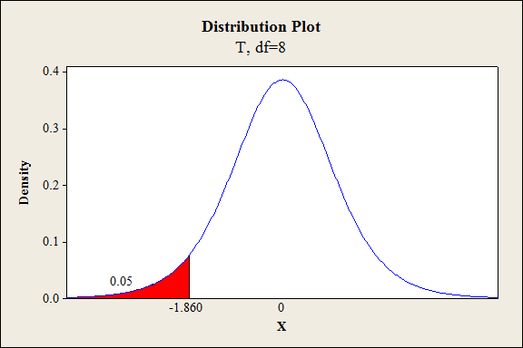
From the output, the critical value is –1.860.
Thus, the critical value is
From the MINITAB output obtained in part (b), the estimate of error standard deviation of slope coefficient is
Test statistic under null hypothesis:
Under the null hypothesis, the test statistic is obtained as follows:
Thus, the test statistic is -0.3931.
Decision criteria for the classical approach:
If
Conclusion:
Here, the test statistic is -0.3931 and critical value is –1.860.
The t statistic is less than the critical value.
That is,
Based on the decision rule, reject the null hypothesis.
Hence, the true average decrease in %total suspended solids removed is not greater than or equal to 0.2.
Therefore, there is no sufficient evidence to infer that the true average decrease in “%total suspended solids removed” associated with 10,000 liters increase in “amount filtered” is greater than or equal to 2.
f.
Find the 95% specified confidence interval for the true mean %total suspended solids removed when the amount filtered is 100,000 liters.
Compare the width of the confidence intervals for 100,000 liters and 200,000 liters amount filtered.
f.
Answer to Problem 48E
The 95% specified confidence interval for the true mean %total suspended solids removed when the amount filtered is 100,000 liters is
The confidence interval for 100,000 liters of amount filtered will be narrower than the interval for 200,000 liters of amount filtered.
Explanation of Solution
Calculation:
From the MINITAB output obtained in part (b), the regression line for the variables %total suspended solids removed
Here, the variable amount filtered
Hence, the value of 100,000 for amount filtered is
Expected %total suspended solids removed when the amount filtered is
The expected value of %total suspended solids removed with
Thus, the expected value of %total suspended solids removed with
Confidence interval:
The general formula for the
Where,
From the MINITAB output in part (a), the value of the standard error of the estimate is
The value of
From the give data, the sum of amount filtered is
The mean amount filtered is,
Thus, the mean amount filtered is
Covariance term
The value of
Thus, the covariance term
Critical value:
For 95% confidence level,
Degrees of freedom:
The sample size is
The degrees of freedom is,
From Table A.5 of the t-distribution in Appendix A, the critical value corresponding to the right tail area 0.025 and 8 degrees of freedom is 2.306.
Thus, the critical value is
The 95% confidence interval is,
Thus, the 95% specified confidence interval for the true mean %total suspended solids removed when the amount filtered is 100,000 liters is
Interpretation:
There is 95% confident that, the true mean %total suspended solids removed when the amount filtered is 100,000 liters lies between 22.37244 and 38.82756.
Comparison:
For 100,000 amount filtered, the value of x is
The mean amount filtered is
Here, the observation
The general formula to obtain
For
For
In the two quantities, the only difference is the values
In general, the value of the quantity
Therefore, the value
The confidence interval will be wider for large value of
Here,
Thus, the confidence interval is wider for
g.
Find the 95% prediction interval for the single value of %total suspended solids removed when the amount filtered is 100,000 liters.
Compare the width of the prediction intervals for 100,000 liters and 200,000 liters amount filtered.
g.
Answer to Problem 48E
The 95% prediction interval for the single value of %total suspended solids removed when the amount filtered is 100,000 liters is
The prediction interval for 100,000 liters of amount filtered will be narrower than the interval for 200,000 liters of amount filtered.
Explanation of Solution
Calculation:
From the MINITAB output obtained in part (b), the regression line for the variables %total suspended solids removed
From part (c), the
Prediction interval for a single future value:
Prediction interval is used to predict a single value of the focus variable that is to be observed at some future time. In other words it can be said that the prediction interval gives a single future value rather than estimating the mean value of the variable.
The general formula for
where
From the MINITAB output in part (b), the value of the standard error of the estimate is
From part (c), the mean chlorine flow is
Critical value:
For 95% confidence level,
Degrees of freedom:
The sample size is
The degrees of freedom is,
From Table A.5 of the t-distribution in Appendix A, the critical value corresponding to the right tail area 0.025 and 8 degrees of freedom is 2.306.
Thus, the critical value is
The 95% prediction interval is,
Thus, the 95% prediction interval for the single value of %total suspended solids removed when the amount filtered is 100,000 liters is
Interpretation:
For repeated samples, there is 95% confident that the single value of % total suspended solids removed when the amount filtered is 100,000 liters will lie between 4.950886 and 56.24911.
Comparison:
For 100,000 amount filtered, the value of x is
The mean amount filtered is
Here, the observation
The general formula to obtain
For
For
In the two quantities, the only difference is the values
In general, the value of the quantity
Therefore, the value
The prediction interval will be wider for large value of
Here,
Thus, the prediction interval is wider for
Want to see more full solutions like this?
Chapter 12 Solutions
Probability and Statistics for Engineering and the Sciences STAT 400 - University Of Maryland


- Bob and Teresa each collect their own samples to test the same hypothesis. Bob’s p-value turns out to be 0.05, and Teresa’s turns out to be 0.01. Why don’t Bob and Teresa get the same p-values? Who has stronger evidence against the null hypothesis: Bob or Teresa?arrow_forwardReview a classmate's Main Post. 1. State if you agree or disagree with the choices made for additional analysis that can be done beyond the frequency table. 2. Choose a measure of central tendency (mean, median, mode) that you would like to compute with the data beyond the frequency table. Complete either a or b below. a. Explain how that analysis can help you understand the data better. b. If you are currently unable to do that analysis, what do you think you could do to make it possible? If you do not think you can do anything, explain why it is not possible.arrow_forward0|0|0|0 - Consider the time series X₁ and Y₁ = (I – B)² (I – B³)Xt. What transformations were performed on Xt to obtain Yt? seasonal difference of order 2 simple difference of order 5 seasonal difference of order 1 seasonal difference of order 5 simple difference of order 2arrow_forward
- Calculate the 90% confidence interval for the population mean difference using the data in the attached image. I need to see where I went wrong.arrow_forwardMicrosoft Excel snapshot for random sampling: Also note the formula used for the last column 02 x✓ fx =INDEX(5852:58551, RANK(C2, $C$2:$C$51)) A B 1 No. States 2 1 ALABAMA Rand No. 0.925957526 3 2 ALASKA 0.372999976 4 3 ARIZONA 0.941323044 5 4 ARKANSAS 0.071266381 Random Sample CALIFORNIA NORTH CAROLINA ARKANSAS WASHINGTON G7 Microsoft Excel snapshot for systematic sampling: xfx INDEX(SD52:50551, F7) A B E F G 1 No. States Rand No. Random Sample population 50 2 1 ALABAMA 0.5296685 NEW HAMPSHIRE sample 10 3 2 ALASKA 0.4493186 OKLAHOMA k 5 4 3 ARIZONA 0.707914 KANSAS 5 4 ARKANSAS 0.4831379 NORTH DAKOTA 6 5 CALIFORNIA 0.7277162 INDIANA Random Sample Sample Name 7 6 COLORADO 0.5865002 MISSISSIPPI 8 7:ONNECTICU 0.7640596 ILLINOIS 9 8 DELAWARE 0.5783029 MISSOURI 525 10 15 INDIANA MARYLAND COLORADOarrow_forwardSuppose the Internal Revenue Service reported that the mean tax refund for the year 2022 was $3401. Assume the standard deviation is $82.5 and that the amounts refunded follow a normal probability distribution. Solve the following three parts? (For the answer to question 14, 15, and 16, start with making a bell curve. Identify on the bell curve where is mean, X, and area(s) to be determined. 1.What percent of the refunds are more than $3,500? 2. What percent of the refunds are more than $3500 but less than $3579? 3. What percent of the refunds are more than $3325 but less than $3579?arrow_forward
- A normal distribution has a mean of 50 and a standard deviation of 4. Solve the following three parts? 1. Compute the probability of a value between 44.0 and 55.0. (The question requires finding probability value between 44 and 55. Solve it in 3 steps. In the first step, use the above formula and x = 44, calculate probability value. In the second step repeat the first step with the only difference that x=55. In the third step, subtract the answer of the first part from the answer of the second part.) 2. Compute the probability of a value greater than 55.0. Use the same formula, x=55 and subtract the answer from 1. 3. Compute the probability of a value between 52.0 and 55.0. (The question requires finding probability value between 52 and 55. Solve it in 3 steps. In the first step, use the above formula and x = 52, calculate probability value. In the second step repeat the first step with the only difference that x=55. In the third step, subtract the answer of the first part from the…arrow_forwardIf a uniform distribution is defined over the interval from 6 to 10, then answer the followings: What is the mean of this uniform distribution? Show that the probability of any value between 6 and 10 is equal to 1.0 Find the probability of a value more than 7. Find the probability of a value between 7 and 9. The closing price of Schnur Sporting Goods Inc. common stock is uniformly distributed between $20 and $30 per share. What is the probability that the stock price will be: More than $27? Less than or equal to $24? The April rainfall in Flagstaff, Arizona, follows a uniform distribution between 0.5 and 3.00 inches. What is the mean amount of rainfall for the month? What is the probability of less than an inch of rain for the month? What is the probability of exactly 1.00 inch of rain? What is the probability of more than 1.50 inches of rain for the month? The best way to solve this problem is begin by a step by step creating a chart. Clearly mark the range, identifying the…arrow_forwardClient 1 Weight before diet (pounds) Weight after diet (pounds) 128 120 2 131 123 3 140 141 4 178 170 5 121 118 6 136 136 7 118 121 8 136 127arrow_forward
- Client 1 Weight before diet (pounds) Weight after diet (pounds) 128 120 2 131 123 3 140 141 4 178 170 5 121 118 6 136 136 7 118 121 8 136 127 a) Determine the mean change in patient weight from before to after the diet (after – before). What is the 95% confidence interval of this mean difference?arrow_forwardIn order to find probability, you can use this formula in Microsoft Excel: The best way to understand and solve these problems is by first drawing a bell curve and marking key points such as x, the mean, and the areas of interest. Once marked on the bell curve, figure out what calculations are needed to find the area of interest. =NORM.DIST(x, Mean, Standard Dev., TRUE). When the question mentions “greater than” you may have to subtract your answer from 1. When the question mentions “between (two values)”, you need to do separate calculation for both values and then subtract their results to get the answer. 1. Compute the probability of a value between 44.0 and 55.0. (The question requires finding probability value between 44 and 55. Solve it in 3 steps. In the first step, use the above formula and x = 44, calculate probability value. In the second step repeat the first step with the only difference that x=55. In the third step, subtract the answer of the first part from the…arrow_forwardIf a uniform distribution is defined over the interval from 6 to 10, then answer the followings: What is the mean of this uniform distribution? Show that the probability of any value between 6 and 10 is equal to 1.0 Find the probability of a value more than 7. Find the probability of a value between 7 and 9. The closing price of Schnur Sporting Goods Inc. common stock is uniformly distributed between $20 and $30 per share. What is the probability that the stock price will be: More than $27? Less than or equal to $24? The April rainfall in Flagstaff, Arizona, follows a uniform distribution between 0.5 and 3.00 inches. What is the mean amount of rainfall for the month? What is the probability of less than an inch of rain for the month? What is the probability of exactly 1.00 inch of rain? What is the probability of more than 1.50 inches of rain for the month? The best way to solve this problem is begin by creating a chart. Clearly mark the range, identifying the lower and upper…arrow_forward
 MATLAB: An Introduction with ApplicationsStatisticsISBN:9781119256830Author:Amos GilatPublisher:John Wiley & Sons Inc
 Probability and Statistics for Engineering and th...StatisticsISBN:9781305251809Author:Jay L. DevorePublisher:Cengage Learning
 Statistics for The Behavioral Sciences (MindTap C...StatisticsISBN:9781305504912Author:Frederick J Gravetter, Larry B. WallnauPublisher:Cengage Learning
 Elementary Statistics: Picturing the World (7th E...StatisticsISBN:9780134683416Author:Ron Larson, Betsy FarberPublisher:PEARSON
 The Basic Practice of StatisticsStatisticsISBN:9781319042578Author:David S. Moore, William I. Notz, Michael A. FlignerPublisher:W. H. Freeman
 Introduction to the Practice of StatisticsStatisticsISBN:9781319013387Author:David S. Moore, George P. McCabe, Bruce A. CraigPublisher:W. H. Freeman