Videos
a.
Find the regression line for the variables fracture toughness
Test whether there is enough evidence to conclude that the predictor variable mode-mixity angle is useful for predicting the value of the response variable fracture toughness.
a.
Answer to Problem 76SE
The regression line for the variables fracture toughness
There is sufficient evidence to conclude that the predictor variable mode-mixity angle is useful for predicting the value of the response variable fracture toughness.
Explanation of Solution
Given info:
The data represents the values of the variables fracture toughness
Calculation:
Linear regression model:
A linear regression model is given as
A linear regression model is given as
Regression:
Software procedure:
Step by step procedure to obtain regression equation using MINITAB software is given as,
- Choose Stat > Regression > Fit Regression Line.
- In Response (Y), enter the column of Fracture toughness.
- In Predictor (X), enter the column of Mode-mixity angle.
- Click OK.
The output using MINITAB software is given as,
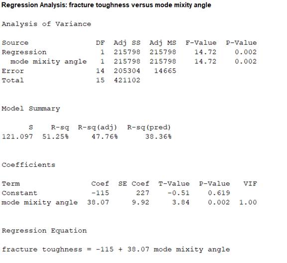
From the MINITAB output, the regression line is
Thus, the regression line for the variables fracture toughness
Interpretation:
The slope estimate implies an increase in fracture toughness by 38.07
The test hypotheses are given below:
Null hypothesis:
That is, there is no useful relationship between the variables fracture toughness
Alternative hypothesis:
That is, there is useful relationship between the variables fracture toughness
T-test statistic:
The test statistic is,
From the MINITAB output, the test statistic is 3.84 and the P-value is 0.002.
Thus, the value of test statistic is 3.84 and P-value is 0.002.
Level of significance:
Here, level of significance is not given.
So, the prior level of significance
Decision rule based on p-value:
If
If
Conclusion:
The P-value is 0.002 and
Here, P-value is less than the
That is
By the rejection rule, reject the null hypothesis.
Thus, there is enough evidence to conclude that the predictor variable mode-mixity angle is useful for predicting the value of the response variable fracture toughness.
b.
Test whether there is enough evidence to conclude that the change in fracture toughness associated with 1 degree increase in mode-mixity angle is greater than 50
b.
Answer to Problem 76SE
There is no sufficient evidence to conclude that the change in fracture toughness associated with 1 degree increase in mode-mixity angle is greater than 50
Explanation of Solution
Calculation:
From the MINITAB output obtained in part (a), the slope coefficient of the regression equation is
Here,
Claim:
Here, the claim is that the true average change in the fracture toughness associated with 1 degree increase in mode-mixity angle is greater than 50
The test hypotheses are given below:
Null hypothesis:
That is, the average change in the fracture toughness associated with 1 degree increase in mode-mixity angle is less than or equal to 50
Alternative hypothesis:
That is, the average change in the fracture toughness associated with 1 degree increase in mode-mixity angle is greater than 50
Test statistic:
The test statistic is,
Degrees of freedom:
The number of concrete beams that are sampled is
The degrees of freedom is,
Thus, the degree of freedom is 14.
Level of significance:
Here, level of significance is not given.
So, the prior level of significance
Critical value:
Software procedure:
Step by step procedure to obtain the critical value using the MINITAB software:
- Choose Graph > Probability Distribution Plot choose View Probability > OK.
- From Distribution, choose ‘t’ distribution and enter 14 as degrees of freedom.
- Click the Shaded Area tab.
- Choose Probability Value and Right Tail for the region of the curve to shade.
- Enter the Probability value as 0.05.
- Click OK.
Output using the MINITAB software is given below:
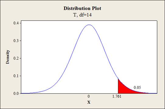
From the output, the critical value is 1.761.
Thus, the critical value is
From the MINITAB output obtained in part (a), the estimate of error standard deviation of slope coefficient is
Test statistic under null hypothesis:
Under the null hypothesis, the test statistic is obtained as follows:
Thus, the test statistic is -1.2026.
Decision criteria for the classical approach:
If
Conclusion:
Here, the test statistic is -1.2026 and critical value is 1.761.
The t statistic is less than the critical value.
That is,
Thus, the decision rule is, failed to reject the null hypothesis.
Hence, the average change in the fracture toughness associated with 1 degree increase in mode-mixity angle is less than or equal to 50
Therefore, there is no sufficient evidence to conclude that the change in fracture toughness associated with 1 degree increase in mode-mixity angle is greater than 50
c.
Explain whether the new observations of the variable mode-mixity angle give more precise estimate of slope coefficient than the actual observations.
c.
Answer to Problem 76SE
No, the new observations of the variable mode-mixity angle do not give more precise estimate of slope coefficient than the actual observations.
Explanation of Solution
Given info:
The data represents the new values of the variable mode-mixity angle, at which the response variable fracture toughness is predicted.
Calculation:
Confidence interval:
The general formula for the confidence interval for the slope of the regression line is,
Where,
The precision of the confidence interval increases with the decrease in the error standard deviation of the slope.
That is, the precision will be high for lower value of
Error sum of square: (SSE)
The variation in the observed values of the response variable that is not explained by the regression is defined as the regression sum of squares. The formula for error sum of square is
Estimate of error standard deviation of slope coefficient:
The general formula for the estimate of error standard deviation of slope coefficient is,
The defining formula for
Here, the estimate of error standard deviation of slope coefficient depends on the value of
The estimate of error standard deviation of slope coefficient decreases with the increase in the value of
The margin of error is product of critical value and standard error of the statistic. The higher width of the confidence interval indicates larger standard error of statistic. Hence, the margin of error also increases.
Therefore, the width of the confidence interval decreases with the decrease in value of error standard deviation. In other words it can be said that the precision decreases with the decrease in the value of
The value of
| 1 | 16.52 | 272.9104 |
| 2 | 17.53 | 307.3009 |
| 3 | 18.05 | 325.8025 |
| 4 | 18.05 | 325.8025 |
| 5 | 22.39 | 501.3121 |
| 6 | 23.89 | 570.7321 |
| 7 | 25.50 | 650.25 |
| 8 | 24.89 | 619.5121 |
| 9 | 23.48 | 551.3104 |
| 10 | 24.98 | 624.0004 |
| 11 | 25.55 | 652.8025 |
| 12 | 25.90 | 670.81 |
| 13 | 22.65 | 513.0225 |
| 14 | 23.69 | 561.2161 |
| 15 | 24.15 | 583.2225 |
| 16 | 24.45 | 597.8025 |
| Total |
Here,
Thus, the value of
Hence, the covariance is
The value of
| 1 | 16 | 256 |
| 2 | 16 | 256 |
| 3 | 18 | 324 |
| 4 | 18 | 324 |
| 5 | 20 | 400 |
| 6 | 20 | 400 |
| 7 | 20 | 400 |
| 8 | 20 | 400 |
| 9 | 22 | 484 |
| 10 | 22 | 484 |
| 11 | 22 | 484 |
| 12 | 22 | 484 |
| 13 | 24 | 576 |
| 14 | 24 | 576 |
| 15 | 26 | 676 |
| 16 | 26 | 676 |
| Total |
Here,
Thus, the value of
Hence, the covariance is
The value of
That is,
Hence, the estimate of error standard deviation of slope coefficient is lower for old observations.
Therefore, the precision is high for old observations.
Thus, the new observations of the variable mode-mixity angle do not give more precise estimate of slope coefficient than the actual observations.
d.
Find the
Find the prediction interval of fracture toughness for a single sandwich panel of 18 degrees mode-mixity angle.
Find the interval estimate for the true mean fracture toughness of all sandwich panels with 22 degrees mode-mixity angle.
Find the prediction interval of fracture toughness for a single sandwich panel of 22 degrees mode-mixity angle.
d.
Answer to Problem 76SE
The 95% specified confidence interval for the true mean fracture toughness of all sandwich panels with 18 degrees mode-mixity angle is
The 95% prediction interval of fracture toughness for a single sandwich panel with 18 degrees mode-mixity angle is
The 95% specified confidence interval for the true mean fracture toughness of all sandwich panels with 22 degrees mode-mixity angle is
The 95% prediction interval of fracture toughness for a single sandwich panel with 22 degrees mode-mixity angle is
Explanation of Solution
Calculation:
Here, the regression equation is
Expected fracture toughness when the mode-mixity angle is 18 degrees:
The expected fracture toughness with 18 degrees mode-mixity angle is obtained as follows:
Thus, the expected fracture toughness with 18 degrees mode-mixity angle is 570.26.
95% confidence interval of true mean fracture tough for an angle of 18 degrees:
The general formula for the
Where,
From the MINITAB output in part (a), the value of the standard error of the estimate is
The value of
| 1 | 16.52 | 272.9104 |
| 2 | 17.53 | 307.3009 |
| 3 | 18.05 | 325.8025 |
| 4 | 18.05 | 325.8025 |
| 5 | 22.39 | 501.3121 |
| 6 | 23.89 | 570.7321 |
| 7 | 25.50 | 650.25 |
| 8 | 24.89 | 619.5121 |
| 9 | 23.48 | 551.3104 |
| 10 | 24.98 | 624.0004 |
| 11 | 25.55 | 652.8025 |
| 12 | 25.90 | 670.81 |
| 13 | 22.65 | 513.0225 |
| 14 | 23.69 | 561.2161 |
| 15 | 24.15 | 583.2225 |
| 16 | 24.45 | 597.8025 |
| Total |
Here,
The mean mode-mixity angle is,
Thus, the mean mode-mixity angle is
Covariance term
Thus, the value of
Hence, the covariance is
Since, the level of confidence is not specified. The prior confidence level 95% can be used.
Critical value:
For 95% confidence level,
Degrees of freedom:
The sample size is
The degrees of freedom is,
From Table A.5 of the t-distribution in Appendix A, the critical value corresponding to the right tail area 0.025 and 14 degrees of freedom is 2.145.
Thus, the critical value is
The 95% confidence interval is,
Thus, the 95% specified confidence interval for the true mean fracture toughness of all sandwich panels with 18 degrees mode-mixity angle is
Interpretation:
There is 95% confident that, the true mean fracture toughness of all sandwich panels with 18 degrees mode-mixity angle lies between 453.6507 and 686.8693.
95% prediction interval of fracture tough for an angle of 18 degrees:
Prediction interval for a single future value:
Prediction interval is used to predict a single value of the focus variable that is to be observed at some future time. In other words it can be said that the prediction interval gives a single future value rather than estimating the mean value of the variable.
The general formula for
where
The 95% prediction interval is,
Thus, the 95% prediction interval of fracture toughness for a single sandwich panel with 18 degrees mode-mixity angle is
Interpretation:
For repeated samples, there is 95% confident that the fracture toughness for a single sandwich panel with 18 degrees mode-mixity angle lies between 285.5331 and 854.9569.
Expected fracture toughness when the mode-mixity angle is 22 degrees:
The expected fracture toughness with 22 degrees mode-mixity angle is obtained as follows:
Thus, the expected fracture toughness with 22 degrees mode-mixity angle is 722.54.
95% confidence interval of true mean fracture tough for an angle of 22 degrees:
The 95% confidence interval is,
Thus, the 95% specified confidence interval for the true mean fracture toughness of all sandwich panels with 22 degrees mode-mixity angle is
Interpretation:
There is 95% confident that, the true mean fracture toughness of all sandwich panels with 22 degrees mode-mixity angle lies between 656.3689 and 788.7111.
95% prediction interval of fracture tough for an angle of 22 degrees:
The 95% prediction interval is,
Thus, the 95% prediction interval of fracture toughness for a single sandwich panel with 22 degrees mode-mixity angle is
Interpretation:
For repeated samples, there is 95% confident that the fracture toughness for a single sandwich panel with 22 degrees mode-mixity angle lies between 454.491 and 990.589.
Want to see more full solutions like this?
Chapter 12 Solutions
Probability and Statistics for Engineering and the Sciences STAT 400 - University Of Maryland


- Calculate the 90% confidence interval for the population mean difference using the data in the attached image. I need to see where I went wrong.arrow_forwardMicrosoft Excel snapshot for random sampling: Also note the formula used for the last column 02 x✓ fx =INDEX(5852:58551, RANK(C2, $C$2:$C$51)) A B 1 No. States 2 1 ALABAMA Rand No. 0.925957526 3 2 ALASKA 0.372999976 4 3 ARIZONA 0.941323044 5 4 ARKANSAS 0.071266381 Random Sample CALIFORNIA NORTH CAROLINA ARKANSAS WASHINGTON G7 Microsoft Excel snapshot for systematic sampling: xfx INDEX(SD52:50551, F7) A B E F G 1 No. States Rand No. Random Sample population 50 2 1 ALABAMA 0.5296685 NEW HAMPSHIRE sample 10 3 2 ALASKA 0.4493186 OKLAHOMA k 5 4 3 ARIZONA 0.707914 KANSAS 5 4 ARKANSAS 0.4831379 NORTH DAKOTA 6 5 CALIFORNIA 0.7277162 INDIANA Random Sample Sample Name 7 6 COLORADO 0.5865002 MISSISSIPPI 8 7:ONNECTICU 0.7640596 ILLINOIS 9 8 DELAWARE 0.5783029 MISSOURI 525 10 15 INDIANA MARYLAND COLORADOarrow_forwardSuppose the Internal Revenue Service reported that the mean tax refund for the year 2022 was $3401. Assume the standard deviation is $82.5 and that the amounts refunded follow a normal probability distribution. Solve the following three parts? (For the answer to question 14, 15, and 16, start with making a bell curve. Identify on the bell curve where is mean, X, and area(s) to be determined. 1.What percent of the refunds are more than $3,500? 2. What percent of the refunds are more than $3500 but less than $3579? 3. What percent of the refunds are more than $3325 but less than $3579?arrow_forward
- A normal distribution has a mean of 50 and a standard deviation of 4. Solve the following three parts? 1. Compute the probability of a value between 44.0 and 55.0. (The question requires finding probability value between 44 and 55. Solve it in 3 steps. In the first step, use the above formula and x = 44, calculate probability value. In the second step repeat the first step with the only difference that x=55. In the third step, subtract the answer of the first part from the answer of the second part.) 2. Compute the probability of a value greater than 55.0. Use the same formula, x=55 and subtract the answer from 1. 3. Compute the probability of a value between 52.0 and 55.0. (The question requires finding probability value between 52 and 55. Solve it in 3 steps. In the first step, use the above formula and x = 52, calculate probability value. In the second step repeat the first step with the only difference that x=55. In the third step, subtract the answer of the first part from the…arrow_forwardIf a uniform distribution is defined over the interval from 6 to 10, then answer the followings: What is the mean of this uniform distribution? Show that the probability of any value between 6 and 10 is equal to 1.0 Find the probability of a value more than 7. Find the probability of a value between 7 and 9. The closing price of Schnur Sporting Goods Inc. common stock is uniformly distributed between $20 and $30 per share. What is the probability that the stock price will be: More than $27? Less than or equal to $24? The April rainfall in Flagstaff, Arizona, follows a uniform distribution between 0.5 and 3.00 inches. What is the mean amount of rainfall for the month? What is the probability of less than an inch of rain for the month? What is the probability of exactly 1.00 inch of rain? What is the probability of more than 1.50 inches of rain for the month? The best way to solve this problem is begin by a step by step creating a chart. Clearly mark the range, identifying the…arrow_forwardClient 1 Weight before diet (pounds) Weight after diet (pounds) 128 120 2 131 123 3 140 141 4 178 170 5 121 118 6 136 136 7 118 121 8 136 127arrow_forward
- Client 1 Weight before diet (pounds) Weight after diet (pounds) 128 120 2 131 123 3 140 141 4 178 170 5 121 118 6 136 136 7 118 121 8 136 127 a) Determine the mean change in patient weight from before to after the diet (after – before). What is the 95% confidence interval of this mean difference?arrow_forwardIn order to find probability, you can use this formula in Microsoft Excel: The best way to understand and solve these problems is by first drawing a bell curve and marking key points such as x, the mean, and the areas of interest. Once marked on the bell curve, figure out what calculations are needed to find the area of interest. =NORM.DIST(x, Mean, Standard Dev., TRUE). When the question mentions “greater than” you may have to subtract your answer from 1. When the question mentions “between (two values)”, you need to do separate calculation for both values and then subtract their results to get the answer. 1. Compute the probability of a value between 44.0 and 55.0. (The question requires finding probability value between 44 and 55. Solve it in 3 steps. In the first step, use the above formula and x = 44, calculate probability value. In the second step repeat the first step with the only difference that x=55. In the third step, subtract the answer of the first part from the…arrow_forwardIf a uniform distribution is defined over the interval from 6 to 10, then answer the followings: What is the mean of this uniform distribution? Show that the probability of any value between 6 and 10 is equal to 1.0 Find the probability of a value more than 7. Find the probability of a value between 7 and 9. The closing price of Schnur Sporting Goods Inc. common stock is uniformly distributed between $20 and $30 per share. What is the probability that the stock price will be: More than $27? Less than or equal to $24? The April rainfall in Flagstaff, Arizona, follows a uniform distribution between 0.5 and 3.00 inches. What is the mean amount of rainfall for the month? What is the probability of less than an inch of rain for the month? What is the probability of exactly 1.00 inch of rain? What is the probability of more than 1.50 inches of rain for the month? The best way to solve this problem is begin by creating a chart. Clearly mark the range, identifying the lower and upper…arrow_forward
- Problem 1: The mean hourly pay of an American Airlines flight attendant is normally distributed with a mean of 40 per hour and a standard deviation of 3.00 per hour. What is the probability that the hourly pay of a randomly selected flight attendant is: Between the mean and $45 per hour? More than $45 per hour? Less than $32 per hour? Problem 2: The mean of a normal probability distribution is 400 pounds. The standard deviation is 10 pounds. What is the area between 415 pounds and the mean of 400 pounds? What is the area between the mean and 395 pounds? What is the probability of randomly selecting a value less than 395 pounds? Problem 3: In New York State, the mean salary for high school teachers in 2022 was 81,410 with a standard deviation of 9,500. Only Alaska’s mean salary was higher. Assume New York’s state salaries follow a normal distribution. What percent of New York State high school teachers earn between 70,000 and 75,000? What percent of New York State high school…arrow_forwardPls help asaparrow_forwardSolve the following LP problem using the Extreme Point Theorem: Subject to: Maximize Z-6+4y 2+y≤8 2x + y ≤10 2,y20 Solve it using the graphical method. Guidelines for preparation for the teacher's questions: Understand the basics of Linear Programming (LP) 1. Know how to formulate an LP model. 2. Be able to identify decision variables, objective functions, and constraints. Be comfortable with graphical solutions 3. Know how to plot feasible regions and find extreme points. 4. Understand how constraints affect the solution space. Understand the Extreme Point Theorem 5. Know why solutions always occur at extreme points. 6. Be able to explain how optimization changes with different constraints. Think about real-world implications 7. Consider how removing or modifying constraints affects the solution. 8. Be prepared to explain why LP problems are used in business, economics, and operations research.arrow_forward
 MATLAB: An Introduction with ApplicationsStatisticsISBN:9781119256830Author:Amos GilatPublisher:John Wiley & Sons Inc
 Probability and Statistics for Engineering and th...StatisticsISBN:9781305251809Author:Jay L. DevorePublisher:Cengage Learning
 Statistics for The Behavioral Sciences (MindTap C...StatisticsISBN:9781305504912Author:Frederick J Gravetter, Larry B. WallnauPublisher:Cengage Learning
 Elementary Statistics: Picturing the World (7th E...StatisticsISBN:9780134683416Author:Ron Larson, Betsy FarberPublisher:PEARSON
 The Basic Practice of StatisticsStatisticsISBN:9781319042578Author:David S. Moore, William I. Notz, Michael A. FlignerPublisher:W. H. Freeman
 Introduction to the Practice of StatisticsStatisticsISBN:9781319013387Author:David S. Moore, George P. McCabe, Bruce A. CraigPublisher:W. H. Freeman