
Concept explainers
Videos
a.
Check whether a linear model is appropriate for the data using the
a.
Answer to Problem 48E
Output using MINITAB software is given below:
Yes, a simple linear model is appropriate for the data.
Explanation of Solution
Given info:
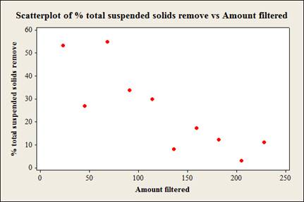
The data represents the values of the variables % total suspended solids removed
Justification:
Software Procedure:
Step by step procedure to obtain scatterplot using MINITAB software is given as,
- Choose Graph > Scatter plot.
- Choose Simple, and then click OK.
- Under Y variables, enter a column of % Total suspended solids removed.
- Under X variables, enter a column of Amount filtered.
- Click Ok.
Observation:
From the scatterplot it is clear that, as the values of amount filtered increases the values of % total suspended solids removed decreases linearly. Thus, there is a negative association between the variables amount filtered and % total suspended solids removed.
Appropriateness of regression linear model:
The conditions for a scatterplot that is well fitted for the data are,
- Straight Enough Condition: The relationship between y and x straight enough to proceed with a linear regression model.
- Outlier Condition: No outlier must be there which influences the fit of the least square line.
- Thickness Condition: The spread of the data around the generally straight relationship seem to be consistent for all values of x.
The scatterplot shows a fair enough linear relationship between the variables amount filtered and % total suspended solids removed. The spread of the data seem to roughly consistent.
Moreover, the scatterplot does not show any outliers.
Therefore, all the three conditions of appropriateness of simple linear model are satisfied.
Thus, a linear model is appropriate for the data.
b.
Find the regression line for the variables % total suspended solids removed
b.
Answer to Problem 48E
The regression line for the variables % total suspended solids removed
Explanation of Solution
Calculation:
Linear regression model:
A linear regression model is given as
A linear regression model is given as
In the given problem the % of total suspended solids remove is the response variable y and the amount filtered is the predictor variable x
Regression:
Software procedure:
Step by step procedure to obtain regression equation using MINITAB software is given as,
- Choose Stat > Regression > Fit Regression Line.
- In Response (Y), enter the column of Removal efficiency.
- In Predictor (X), enter the column of Inlet temperature.
- Click OK.
The output using MINITAB software is given as,
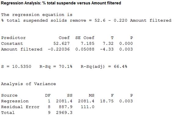
Thus, the regression line for the variables % total suspended solids removed
Interpretation:
The slope estimate implies a decrease in % total suspended solids removed by 22.0% for every 1,000 liters increase in amount filtered. It can also be said that, for every 1% increase in amount filtered the % total suspended solids removed decreases 22%.
c.
Find the proportion of observed variation in % total suspended solids removed that can be explained by amount filtered using the simple linear regression model.
c.
Answer to Problem 48E
The proportion of observed variation in % total suspended solids removed that can be explained by amount filtered using the simple linear regression model is
Explanation of Solution
Justification:
The coefficient of determination (
The general formula to obtain coefficient of variation is,
From the regression output obtained in part (b), the value of coefficient of determination is 0.701.
Thus, the coefficient of determination is
Interpretation:
From this coefficient of determination it can be said that, the amount filtered can explain only 70.1% variability in % total suspended solids removed. Then remaining variability of % total suspended solids removed is explained by other variables.
Thus, the percentage of variation in the observed values of %total suspended solids removed that is explained by the regression is 70.1%, which indicates that 70.1% of the variability in %total suspended solids removed is explained by variability in the amount filtered using the linear regression model.
d.
Test whether there is enough evidence to conclude that the predictor variable amount filtered is useful for predicting the value of the response variable %total suspended solids removed at
d.
Answer to Problem 48E
There is sufficient evidence to conclude that the predictor variable amount filtered is useful for predicting the value of the response variable %total suspended solids removed.
Explanation of Solution
Calculation:
From the MINITAB output obtained in part (b), the regression line for the variables %total suspended solids removed
The test hypotheses are given below:
Null hypothesis:
That is, there is no useful relationship between the variables %total suspended solids removed
Alternative hypothesis:
That is, there is useful relationship between the variables %total suspended solids removed
T-test statistic:
The test statistic is,
From the MINITAB output obtained in part (b), the test statistic is -4.33 and the P-value is 0.003.
Thus, the value of test statistic is -4.33 and P-value is 0.003.
Level of significance:
Here, level of significance is
Decision rule based on p-value:
If
If
Conclusion:
The P-value is 0.003 and
Here, P-value is less than the
That is
By the rejection rule, reject the null hypothesis.
Thus, there is sufficient evidence to conclude that the predictor variable amount filtered is useful for predicting the value of the response variable %total suspended solids removed.
e.
Test whether there is enough evidence to infer that the true average decrease in “%total suspended solids removed” associated with 10,000 liters increase in “amount filtered” is greater than or equal to 2 at
e.
Answer to Problem 48E
There is no sufficient evidence to infer that the true average decrease in “%total suspended solids removed” associated with 10,000 liters increase in “amount filtered” is greater than or equal to 2.
Explanation of Solution
Calculation:
Linear regression model:
A linear regression model is given as
A linear regression model is given as
From the MINITAB output in part (b), the slope coefficient of the regression equation is
Here,
Here, the claim is that, when the amount filtered is increased from 10,000 liters the true average decrease in %total suspended solids removed is greater than or equal to 2.
The claim states that, amount filtered is increased by 10,000 liters.
Decrease in the %total suspended solids removed for 1,000 liters increase in amount filtered:
The true average decrease in the %total suspended solids removed for 1,000 liters increase in amount filtered is,
That is, when the amount filtered is increased by 1,000 liters the true average decrease in %total suspended solids removed is greater than or equal to 0.2.
The test hypotheses are given below:
Null hypothesis:
That is, the true average decrease in %total suspended solids removed is greater than or equal to 0.2.
Alternative hypothesis:
That is, the true average decrease in %total suspended solids removed is less than 0.2.
Test statistic:
The test statistic is,
Degrees of freedom:
The sample size is
The degrees of freedom is,
Thus, the degree of freedom is 8.
Here, level of significance is
Critical value:
Software procedure:
Step by step procedure to obtain the critical value using the MINITAB software:
- Choose Graph > Probability Distribution Plot choose View Probability > OK.
- From Distribution, choose ‘t’ distribution and enter 8 as degrees of freedom.
- Click the Shaded Area tab.
- Choose Probability Value and Left Tail for the region of the curve to shade.
- Enter the Probability value as 0.05.
- Click OK.
Output using the MINITAB software is given below:
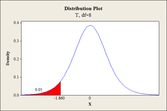
From the output, the critical value is –1.860.
Thus, the critical value is
From the MINITAB output obtained in part (b), the estimate of error standard deviation of slope coefficient is
Test statistic under null hypothesis:
Under the null hypothesis, the test statistic is obtained as follows:
Thus, the test statistic is -0.3931.
Decision criteria for the classical approach:
If
Conclusion:
Here, the test statistic is -0.3931 and critical value is –1.860.
The t statistic is less than the critical value.
That is,
Based on the decision rule, reject the null hypothesis.
Hence, the true average decrease in %total suspended solids removed is not greater than or equal to 0.2.
Therefore, there is no sufficient evidence to infer that the true average decrease in “%total suspended solids removed” associated with 10,000 liters increase in “amount filtered” is greater than or equal to 2.
f.
Find the 95% specified confidence interval for the true mean %total suspended solids removed when the amount filtered is 100,000 liters.
Compare the width of the confidence intervals for 100,000 liters and 200,000 liters amount filtered.
f.
Answer to Problem 48E
The 95% specified confidence interval for the true mean %total suspended solids removed when the amount filtered is 100,000 liters is
The confidence interval for 100,000 liters of amount filtered will be narrower than the interval for 200,000 liters of amount filtered.
Explanation of Solution
Calculation:
From the MINITAB output obtained in part (b), the regression line for the variables %total suspended solids removed
Here, the variable amount filtered
Hence, the value of 100,000 for amount filtered is
Expected %total suspended solids removed when the amount filtered is
The expected value of %total suspended solids removed with
Thus, the expected value of %total suspended solids removed with
Confidence interval:
The general formula for the
Where,
From the MINITAB output in part (a), the value of the standard error of the estimate is
The value of
From the give data, the sum of amount filtered is
The mean amount filtered is,
Thus, the mean amount filtered is
Covariance term
The value of
Thus, the covariance term
Critical value:
For 95% confidence level,
Degrees of freedom:
The sample size is
The degrees of freedom is,
From Table A.5 of the t-distribution in Appendix A, the critical value corresponding to the right tail area 0.025 and 8 degrees of freedom is 2.306.
Thus, the critical value is
The 95% confidence interval is,
Thus, the 95% specified confidence interval for the true mean %total suspended solids removed when the amount filtered is 100,000 liters is
Interpretation:
There is 95% confident that, the true mean %total suspended solids removed when the amount filtered is 100,000 liters lies between 22.37244 and 38.82756.
Comparison:
For 100,000 amount filtered, the value of x is
The mean amount filtered is
Here, the observation
The general formula to obtain
For
For
In the two quantities, the only difference is the values
In general, the value of the quantity
Therefore, the value
The confidence interval will be wider for large value of
Here,
Thus, the confidence interval is wider for
g.
Find the 95% prediction interval for the single value of %total suspended solids removed when the amount filtered is 100,000 liters.
Compare the width of the prediction intervals for 100,000 liters and 200,000 liters amount filtered.
g.
Answer to Problem 48E
The 95% prediction interval for the single value of %total suspended solids removed when the amount filtered is 100,000 liters is
The prediction interval for 100,000 liters of amount filtered will be narrower than the interval for 200,000 liters of amount filtered.
Explanation of Solution
Calculation:
From the MINITAB output obtained in part (b), the regression line for the variables %total suspended solids removed
From part (c), the
Prediction interval for a single future value:
Prediction interval is used to predict a single value of the focus variable that is to be observed at some future time. In other words it can be said that the prediction interval gives a single future value rather than estimating the mean value of the variable.
The general formula for
where
From the MINITAB output in part (b), the value of the standard error of the estimate is
From part (c), the mean chlorine flow is
Critical value:
For 95% confidence level,
Degrees of freedom:
The sample size is
The degrees of freedom is,
From Table A.5 of the t-distribution in Appendix A, the critical value corresponding to the right tail area 0.025 and 8 degrees of freedom is 2.306.
Thus, the critical value is
The 95% prediction interval is,
Thus, the 95% prediction interval for the single value of %total suspended solids removed when the amount filtered is 100,000 liters is
Interpretation:
For repeated samples, there is 95% confident that the single value of % total suspended solids removed when the amount filtered is 100,000 liters will lie between 4.950886 and 56.24911.
Comparison:
For 100,000 amount filtered, the value of x is
The mean amount filtered is
Here, the observation
The general formula to obtain
For
For
In the two quantities, the only difference is the values
In general, the value of the quantity
Therefore, the value
The prediction interval will be wider for large value of
Here,
Thus, the prediction interval is wider for
Want to see more full solutions like this?
Chapter 12 Solutions
Probability and Statistics for Engineering and the Sciences


- The following relates to Problems 4 and 5. Christchurch, New Zealand experienced a major earthquake on February 22, 2011. It destroyed 100,000 homes. Data were collected on a sample of 300 damaged homes. These data are saved in the file called CIEG315 Homework 4 data.xlsx, which is available on Canvas under Files. A subset of the data is shown in the accompanying table. Two of the variables are qualitative in nature: Wall construction and roof construction. Two of the variables are quantitative: (1) Peak ground acceleration (PGA), a measure of the intensity of ground shaking that the home experienced in the earthquake (in units of acceleration of gravity, g); (2) Damage, which indicates the amount of damage experienced in the earthquake in New Zealand dollars; and (3) Building value, the pre-earthquake value of the home in New Zealand dollars. PGA (g) Damage (NZ$) Building Value (NZ$) Wall Construction Roof Construction Property ID 1 0.645 2 0.101 141,416 2,826 253,000 B 305,000 B T 3…arrow_forwardRose Par posted Apr 5, 2025 9:01 PM Subscribe To: Store Owner From: Rose Par, Manager Subject: Decision About Selling Custom Flower Bouquets Date: April 5, 2025 Our shop, which prides itself on selling handmade gifts and cultural items, has recently received inquiries from customers about the availability of fresh flower bouquets for special occasions. This has prompted me to consider whether we should introduce custom flower bouquets in our shop. We need to decide whether to start offering this new product. There are three options: provide a complete selection of custom bouquets for events like birthdays and anniversaries, start small with just a few ready-made flower arrangements, or do not add flowers. There are also three possible outcomes. First, we might see high demand, and the bouquets could sell quickly. Second, we might have medium demand, with a few sold each week. Third, there might be low demand, and the flowers may not sell well, possibly going to waste. These outcomes…arrow_forwardConsider the state space model X₁ = §Xt−1 + Wt, Yt = AX+Vt, where Xt Є R4 and Y E R². Suppose we know the covariance matrices for Wt and Vt. How many unknown parameters are there in the model?arrow_forward
- Business Discussarrow_forwardYou want to obtain a sample to estimate the proportion of a population that possess a particular genetic marker. Based on previous evidence, you believe approximately p∗=11% of the population have the genetic marker. You would like to be 90% confident that your estimate is within 0.5% of the true population proportion. How large of a sample size is required?n = (Wrong: 10,603) Do not round mid-calculation. However, you may use a critical value accurate to three decimal places.arrow_forward2. [20] Let {X1,..., Xn} be a random sample from Ber(p), where p = (0, 1). Consider two estimators of the parameter p: 1 p=X_and_p= n+2 (x+1). For each of p and p, find the bias and MSE.arrow_forward
- 1. [20] The joint PDF of RVs X and Y is given by xe-(z+y), r>0, y > 0, fx,y(x, y) = 0, otherwise. (a) Find P(0X≤1, 1arrow_forward4. [20] Let {X1,..., X} be a random sample from a continuous distribution with PDF f(x; 0) = { Axe 5 0, x > 0, otherwise. where > 0 is an unknown parameter. Let {x1,...,xn} be an observed sample. (a) Find the value of c in the PDF. (b) Find the likelihood function of 0. (c) Find the MLE, Ô, of 0. (d) Find the bias and MSE of 0.arrow_forward3. [20] Let {X1,..., Xn} be a random sample from a binomial distribution Bin(30, p), where p (0, 1) is unknown. Let {x1,...,xn} be an observed sample. (a) Find the likelihood function of p. (b) Find the MLE, p, of p. (c) Find the bias and MSE of p.arrow_forwardGiven the sample space: ΩΞ = {a,b,c,d,e,f} and events: {a,b,e,f} A = {a, b, c, d}, B = {c, d, e, f}, and C = {a, b, e, f} For parts a-c: determine the outcomes in each of the provided sets. Use proper set notation. a. (ACB) C (AN (BUC) C) U (AN (BUC)) AC UBC UCC b. C. d. If the outcomes in 2 are equally likely, calculate P(AN BNC).arrow_forwardSuppose a sample of O-rings was obtained and the wall thickness (in inches) of each was recorded. Use a normal probability plot to assess whether the sample data could have come from a population that is normally distributed. Click here to view the table of critical values for normal probability plots. Click here to view page 1 of the standard normal distribution table. Click here to view page 2 of the standard normal distribution table. 0.191 0.186 0.201 0.2005 0.203 0.210 0.234 0.248 0.260 0.273 0.281 0.290 0.305 0.310 0.308 0.311 Using the correlation coefficient of the normal probability plot, is it reasonable to conclude that the population is normally distributed? Select the correct choice below and fill in the answer boxes within your choice. (Round to three decimal places as needed.) ○ A. Yes. The correlation between the expected z-scores and the observed data, , exceeds the critical value, . Therefore, it is reasonable to conclude that the data come from a normal population. ○…arrow_forwardding question ypothesis at a=0.01 and at a = 37. Consider the following hypotheses: 20 Ho: μ=12 HA: μ12 Find the p-value for this hypothesis test based on the following sample information. a. x=11; s= 3.2; n = 36 b. x = 13; s=3.2; n = 36 C. c. d. x = 11; s= 2.8; n=36 x = 11; s= 2.8; n = 49arrow_forwardarrow_back_iosSEE MORE QUESTIONSarrow_forward_ios
 MATLAB: An Introduction with ApplicationsStatisticsISBN:9781119256830Author:Amos GilatPublisher:John Wiley & Sons Inc
 Probability and Statistics for Engineering and th...StatisticsISBN:9781305251809Author:Jay L. DevorePublisher:Cengage Learning
 Statistics for The Behavioral Sciences (MindTap C...StatisticsISBN:9781305504912Author:Frederick J Gravetter, Larry B. WallnauPublisher:Cengage Learning
 Elementary Statistics: Picturing the World (7th E...StatisticsISBN:9780134683416Author:Ron Larson, Betsy FarberPublisher:PEARSON
 The Basic Practice of StatisticsStatisticsISBN:9781319042578Author:David S. Moore, William I. Notz, Michael A. FlignerPublisher:W. H. Freeman
 Introduction to the Practice of StatisticsStatisticsISBN:9781319013387Author:David S. Moore, George P. McCabe, Bruce A. CraigPublisher:W. H. Freeman