Statistics: The Art and Science of Learning from Data (4th Edition)
4th Edition
ISBN: 9780321997838
Author: Alan Agresti, Christine A. Franklin, Bernhard Klingenberg
Publisher: PEARSON
expand_more
expand_more
format_list_bulleted
Concept explainers
Videos
Textbook Question
Chapter 12.4, Problem 47PB
ANOVA table for leg press Exercise 12.15 referred to an analysis of leg strength for 57 female athletes, with y = maximum leg press and x = number of 200-pound leg presses until fatigue, for which
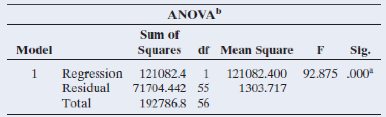
- a. Show that the residual standard deviation is 36.1. Interpret it.
- b. For this sample, x̄ = 22.2. For female athletes with x = 22, what would you estimate the variability to be of their maximum leg press values? If the y values are approximately normal, find an interval within which about 95% of them would fall.
Expert Solution & Answer
Want to see the full answer?
Check out a sample textbook solution
Students have asked these similar questions
The mean travel time from one stop to the next on the Coast Starlight Amtrak is 129 minutes, with a standard deviation of 113 minutes. The mean distance travelled from one stop to the next is 108 miles with standard deviation of 99 miles. The correlation between travel time and distance is 0.636.
a). Find the equation of the regression line for predicting travel time.
A sample of 100 bears was treated like it was the whole population of Jellystone Park bears, and the mean weight was found to be 800 pounds with standard deviation 12 pounds, the mean blood pressure was 150 with standard deviation 6, and the sample correlation coefficient of weight with blood pressure was found to be .4. Based on this information, what is the regression slope for the SLR equation for predicting blood pressure using observed weight for Jellystone bears?
a sample of 60 grade 9 student age was obtained to estimate the mean age of all grade 9 students. x = 15.3 years and the population variance is 16
Chapter 12 Solutions
Statistics: The Art and Science of Learning from Data (4th Edition)
Ch. 12.1 - Car mileage and weight The Car Weight and Mileage...Ch. 12.1 - Prob. 2PBCh. 12.1 - Predicting maximum bench strength in males For the...Ch. 12.1 - Prob. 4PBCh. 12.1 - Mu, not y For a population regression equation,...Ch. 12.1 - Prob. 6PBCh. 12.1 - Study time and college GPA Exercise 3.39 in...Ch. 12.1 - Prob. 8PBCh. 12.1 - Cell phone specs Refer to the cell phone data set...Ch. 12.1 - Prob. 10PB
Ch. 12.2 - t-score? A regression analysis is conducted with...Ch. 12.2 - Prob. 12PBCh. 12.2 - Confidence interval for slope Refer to the...Ch. 12.2 - Prob. 14PBCh. 12.2 - Strength through leg press The high school female...Ch. 12.2 - Prob. 16PBCh. 12.2 - More girls are good? Repeat the previous exercise...Ch. 12.2 - CI and two-sided tests correspond Refer to the...Ch. 12.2 - Advertising and sales Each month, the owner of Caf...Ch. 12.2 - Prob. 20PBCh. 12.2 - GPA and skipping classrevisited Refer to the...Ch. 12.2 - Prob. 22PBCh. 12.3 - Dollars and thousands of dollars If a slope is...Ch. 12.3 - Prob. 24PBCh. 12.3 - Sketch scatterplot Sketch a scatterplot,...Ch. 12.3 - Prob. 26PBCh. 12.3 - Body fat For the Male Athlete Strength data file...Ch. 12.3 - Prob. 28PBCh. 12.3 - SAT regression toward mean Refer to the previous...Ch. 12.3 - Prob. 30PBCh. 12.3 - GPA and study time Refer to the association you...Ch. 12.3 - Prob. 32PBCh. 12.3 - Does tutoring help? For a class of 100 students,...Ch. 12.3 - Prob. 34PBCh. 12.3 - Golf regression In the first round of a golf...Ch. 12.3 - Prob. 36PBCh. 12.3 - Food and drink sales The owner of Berthas...Ch. 12.3 - Prob. 38PBCh. 12.3 - Violent crime and single-parent families Use...Ch. 12.4 - Poor predicted strengths The MINITAB output shows...Ch. 12.4 - Prob. 42PBCh. 12.4 - Bench press residuals The figure is a histogram of...Ch. 12.4 - Predicting house prices The House Selling Prices...Ch. 12.4 - Predicting clothes purchases For a random sample...Ch. 12.4 - Prob. 46PBCh. 12.4 - ANOVA table for leg press Exercise 12.15 referred...Ch. 12.4 - Prob. 48PBCh. 12.4 - Variability and F Refer to the previous two...Ch. 12.4 - Understanding an ANOVA table For a random sample...Ch. 12.4 - Predicting cell phone weight Refer to the cell...Ch. 12.4 - Cell phone ANOVA Report the ANOVA table for the...Ch. 12.5 - Savings grow exponentially You invest 100 in a...Ch. 12.5 - Prob. 55PBCh. 12.5 - Prob. 56PBCh. 12.5 - Prob. 57PBCh. 12.5 - Prob. 58PBCh. 12.5 - Prob. 59PBCh. 12.5 - Prob. 60PBCh. 12.5 - Prob. 61PBCh. 12 - Prob. 62CPCh. 12 - Prob. 63CPCh. 12 - Prob. 64CPCh. 12 - Prob. 65CPCh. 12 - Prob. 66CPCh. 12 - Prob. 67CPCh. 12 - Prob. 68CPCh. 12 - Prob. 69CPCh. 12 - Prob. 70CPCh. 12 - Prob. 71CPCh. 12 - Prob. 72CPCh. 12 - Prob. 73CPCh. 12 - Prob. 74CPCh. 12 - World population growth The table shows the world...Ch. 12 - Prob. 76CPCh. 12 - Prob. 77CPCh. 12 - Prob. 78CPCh. 12 - Prob. 79CPCh. 12 - Prob. 81CPCh. 12 - Prob. 82CPCh. 12 - Prob. 83CPCh. 12 - Prob. 84CPCh. 12 - Prob. 85CPCh. 12 - Prob. 86CPCh. 12 - Prob. 87CPCh. 12 - Prob. 88CPCh. 12 - Prob. 89CPCh. 12 - Assumptions What assumptions are needed to use the...Ch. 12 - Assumptions fail? Refer to the previous exercise....Ch. 12 - Lots of standard deviations Explain carefully the...Ch. 12 - Decrease in home values A Freddie Mac quarterly...Ch. 12 - Population growth Exercise 12.57 about U.S....Ch. 12 - Multiple choice: Interpret r One can interpret r =...Ch. 12 - Multiple choice: Correlation invalid The...Ch. 12 - Multiple choice: Slope and correlation The slope...Ch. 12 - Multiple choice: Regress x on y The regression of...Ch. 12 - Multiple choice: Income and height University of...Ch. 12 - True or false The variables y = annual income...Ch. 12 - Prob. 101CPCh. 12 - Why is there regression toward the mean? Refer to...Ch. 12 - Prob. 103CPCh. 12 - Prob. 104CPCh. 12 - Prob. 105CPCh. 12 - Prob. 106CP
Knowledge Booster


Learn more about
Need a deep-dive on the concept behind this application? Look no further. Learn more about this topic, statistics and related others by exploring similar questions and additional content below.Similar questions
- Listed below are the overhead widths (cm) of seals measured from photographs and weights (kg) of the seals. Find the regression equation, letting the overhead width be the predictor (x) variable. Find the best predicted weight of a seal if the overhead width measured from a photograph is1.8cm, using the regression equation. Can the prediction be correct? If not, what is wrong? Use a significance level of 0.05. Overhead_Width_(cm) Weight_(kg)7.2 1287.4 1679.8 2619.5 2218.7 2118.3 201 The regression equation is y=enter your response here+enter your response herex. (Round the y-intercept to the nearest integer as needed. Round the slope to one decimal place as needed.) Part 2 The best predicted weight for an overhead width of 1.8 cm, based on the regression equation, is enter your response here kg. (Round to one decimal place as needed.) Part 3 Can the prediction be correct? If not, what is wrong? A. The prediction cannot be correct…arrow_forwardI have an 1800 square foot home and based on median price of 628,408, mean listing price $401,398, standard deviation $168,408 and median sq foot of 2108, mean sq foot 2295 and standard deviation sq foot 1128, how do I calculate the regression equation to come up with a listing price for and 1800 sqft home?arrow_forwardAn exam score has a mean of 504 and standard deviation of 90. What exam score coresponds to a Z-score of 1.60?arrow_forward
- Unfortunately, arsenic occurs naturally in some ground water. A mean arsenic level of m= 8.0 parts per billion (ppb) is considered safe for agricultural use. A well in Texas is used to water cotton crops. This well is tested on a regular basis for arsenic. A random sample of 37 tests gave a sample mean of xbar= 7.2 ppb arsenic, with s= 1.9 ppb. Does this info indicate that the mean level of arsenic in this well is less than 8ppb? Use a= 0.01. Show full detail.arrow_forwardCerebral blood flow (CBF) in the brains of healthy people is normally distributed with a mean of 74 and a standard deviation of 16. Find the Z score associated with a CBF reading of 78.arrow_forwardAvalanches can be a real problem for travelers in the western United States and Canada. Slab avalanches studied in Canada had an average thickness of u = 67 cm. A sample of 31 avalanches in the U.S. gave a sample mean of = 63.0 cm. It is known that o = 10.3 cm for this type of data. Use a 0.03 level of significance to test the claim that the mean slab thickness of avalanches in the United States is different from that in Canada. Use the P-Value Approach. What are the hypotheses for this problem? А: Но и 3D 63.0 ст us На и + 63.0 ст B: Но и 63.0 ст С: Но и %3D 67 ст us HA и < 67 ст D: Ho u = 67 cm vs HA H# 67 cm B O Aarrow_forward
- Avalanches can be a real problem for travelers in the western United States and Canada. Slab avalanches studied in Canada had an average thickness of µ = 67 cm. A sample of 31 avalanches in the U.S. gave a sample mean of = 63.0 cm. It is known that o = 10.3 cm for this type of data. Use a 0.03 level of significance to test the claim that the mean slab thickness of avalanches in the United States is different from that in Canada. Use the P-Value Approach. What is the Decision for this problem? O There is not sufficient evidence at the 0.03 level of significance to show that the mean slab thickness of avalanches in the United States is different from that in Canada. There is sufficient evidence at the 0.03 level of significance to show that the mean slab thickness of avalanches in the United States is less than that in Canada. There is sufficient evidence at the 0.03 level of significance to show that the mean slab thickness of avalanches in the United States is different from that in…arrow_forwardThe sample mean of depression scores of 16 fifth graders was 4.4 with standard deviation of 8. If the population mean of this depression score is 6, what is the calculated t score for this sample?arrow_forwardThe distribution for the time a patient of a medical center spends waiting for an appointment is normal with mean of 35 minutes and standard deviation of 12 minutes. What percentage of patients will wait less than or equal to 40 minutes for an appointment?arrow_forward
- Based on the scatter plot above, describe the relationship between the amount of cost damage and the distance from nearest fire station to the residential. Determine the regression line for the above regression output. Interpret the slope coefficient of distance to the nearest station affecting the amount of fire cost damage. Compute the correlation coefficient and interpret its meaning. Does the distance to the nearest fire station has significant influence on the cost damage amount? Conduct a test at 1% significance level. ] Predict the fire cost damage generated if the distance from nearest fire station is 2.5 kilometers. Is this estimate reliable? Explain. []arrow_forwarda residual is the distance between the data value in the line of best fit true or false?arrow_forwardThe amount of coffee dispensed by a coffee dispensing machine is normally distributed with mean of 190 mL and a standard deviation of 10 mL. What percentage of the coffee dispensed over 175 ml?arrow_forward
arrow_back_ios
SEE MORE QUESTIONS
arrow_forward_ios
Recommended textbooks for you
 Glencoe Algebra 1, Student Edition, 9780079039897...AlgebraISBN:9780079039897Author:CarterPublisher:McGraw Hill
 Big Ideas Math A Bridge To Success Algebra 1: Stu...AlgebraISBN:9781680331141Author:HOUGHTON MIFFLIN HARCOURTPublisher:Houghton Mifflin Harcourt
Glencoe Algebra 1, Student Edition, 9780079039897...
Algebra
ISBN:9780079039897
Author:Carter
Publisher:McGraw Hill
Big Ideas Math A Bridge To Success Algebra 1: Stu...
Algebra
ISBN:9781680331141
Author:HOUGHTON MIFFLIN HARCOURT
Publisher:Houghton Mifflin Harcourt
Correlation Vs Regression: Difference Between them with definition & Comparison Chart; Author: Key Differences;https://www.youtube.com/watch?v=Ou2QGSJVd0U;License: Standard YouTube License, CC-BY
Correlation and Regression: Concepts with Illustrative examples; Author: LEARN & APPLY : Lean and Six Sigma;https://www.youtube.com/watch?v=xTpHD5WLuoA;License: Standard YouTube License, CC-BY