Chapter 12.2, Problem 16E

The race for the 2013 Academy Award for Actress in a Leading Role was extremely tight, featuring several worthy performances (ABC News online, February 22, 2013). The nominees were Jessica Chastain for Zero Dark thirty, Jennifer Lawrence for Silver Linings Playbook, Emmanuelle Riva for Amour, Quvenzhané Wallis for Beasts of the Southern Wild, and Naomi Watts for the Impossible. In a survey, movie fans who had seen each of the movies for which these five actresses had been nominated were asked to select the actress who was most deserving of the 2013 Academy Award for Actress in a Leading Role. The responses follow.

	18–30	31–4	45–58	Over 58
Jessica Chastain	51	50	41	42
Jennifer Lawrence	63	55	37	50
Emmanuelle Riva	15	44	56	74
Quvenzhané Wallis	48	25	22	31
Naomi Watts	36	65	62	33

1. a. How large was the sample in this survey?
2. b. Jennifer Lawrence received the 2013 Academy Award for Actress in a Leading Role for her performance in Silver Linings Playbook. Did the respondents favor Ms. Lawrence? c. at α = .05, conduct a hypothesis test to determine whether people’s attitude toward the actress who was most deserving of the 2013 Academy Award for Actress in a Leading Role is independent of respondent age. What is your Conclusion?

To determine

Find the sample size for the given survey.

Answer to Problem 16E

The sample size is 900.

Explanation of Solution

Calculation:

The given observed frequency $\left(f_{ij}\right)$ as the row and column total is tabulated below:

Actress	Age 18-30	Age 31-44	Age 45-58	Age over 58	Total
Jessica Chastain	51	50	41	42	184
Jennifer Lawrence	63	55	37	50	205
Emmanuelle Riva	15	44	56	74	189
Quvenzhane Wallis	48	25	22	31	126
Naomi Watts	36	65	62	33	196
Total	213	239	218	230	900

Thus, the sample size is 900.

To determine

Explain whether the respondents favor Ms. Lawrence.

Explanation of Solution

Calculation:

Jennifer Lawrence received the 2013 Academy Award for actress in a leading role for “Silver Lining Playbook”.

The sample proportion of movie fan for Jessica Chastain is,

$\begin{array}{c}\overline{p_1}=\frac{184}{900}\\ =0.2044\end{array}$

The sample proportion of movie fan for Jennifer Lawrence is,

$\begin{array}{c}\overline{p_2}=\frac{205}{900}\\ =0.2278\end{array}$

The sample proportion of movie fan for Emmanuelle Riva is,

$\begin{array}{c}\overline{p_3}=\frac{189}{900}\\ =0.2100\end{array}$

The sample proportion of movie fan for Quvenzhane Wallis is,

$\begin{array}{c}\overline{p_4}=\frac{126}{900}\\ =0.1400\end{array}$

The sample proportion of movie fan for Naomi Watts is,

$\begin{array}{c}\overline{p_5}=\frac{196}{900}\\ =0.2178\end{array}$

It is clear that, the sample proportion for Jennifer Lawrence is highest. Thus, the respondents favor Ms. Lawrence. However, Jessica Chastain, Emmanuelle Riva and Naomi Watts were also favored by almost as many of fans.

To determine

Perform a hypothesis test to determine whether people’s attitude toward the actress who was most deserving of the 2013 Academy Award for Actress in a Leading Role is independent of respondent age at 5% level of significance and draw conclusion of the study.

Answer to Problem 16E

The data provide sufficient evidence to conclude that people’s attitude toward the actress who was most deserving of the 2013 Academy Award for Actress in a Leading Role is not independent of respondent age.

Explanation of Solution

Calculation:

State the test hypotheses.

Null hypothesis:

$H_0:\text{The two cataegorical variables are independent}$

That is, people’s attitude toward the actress who was most deserving of the 2013 Academy Award for Actress in a Leading Role is independent of respondent age.

Alternative hypothesis:

$H_a:\text{The two cataegorical variables are not independent}$

That is, people’s attitude toward the actress who was most deserving of the 2013 Academy Award for Actress in a Leading Role is not independent of respondent age.

The row and column total is tabulated below:

Actress	Age 18-30	Age 31-44	Age 45-58	Age over 58	Total
Jessica Chastain	51	50	41	42	184
Jennifer Lawrence	63	55	37	50	205
Emmanuelle Riva	15	44	56	74	189
Quvenzhane Wallis	48	25	22	31	126
Naomi Watts	36	65	62	33	196
Totals	213	239	218	230	900

The formula for expected frequency is given below:

$e_{ij}=\frac{\left(\text{Row }i\text{ Total}\right)\left(\text{Coloumn }j\text{ Total}\right)}{\text{Total Sample Size}}$

The expected frequency for each category is calculated as follows:

Actress	Age 18-30	Age 31-44	Age 45-58	Age over 58
Jessica Chastain	$\begin{array}{l}\frac{\left(184\right)\left(213\right)}{900}\\ =43.5\end{array}$	$\begin{array}{l}\frac{\left(184\right)\left(239\right)}{900}\\ =48.9\end{array}$	$\begin{array}{l}\frac{\left(184\right)\left(218\right)}{900}\\ =44.6\end{array}$	$\begin{array}{l}\frac{\left(184\right)\left(230\right)}{900}\\ =47\end{array}$
Jennifer Lawrence	$\begin{array}{l}\frac{\left(205\right)\left(213\right)}{900}\\ =48.5\end{array}$	$\begin{array}{l}\frac{\left(205\right)\left(239\right)}{900}\\ =54.4\end{array}$	$\begin{array}{l}\frac{\left(205\right)\left(218\right)}{900}\\ =49.7\end{array}$	$\begin{array}{l}\frac{\left(205\right)\left(230\right)}{900}\\ =52.4\end{array}$
Emmanuelle Riva	$\begin{array}{l}\frac{\left(189\right)\left(213\right)}{900}\\ =29.8\end{array}$	$\begin{array}{l}\frac{\left(189\right)\left(239\right)}{900}\\ =50.2\end{array}$	$\begin{array}{l}\frac{\left(189\right)\left(218\right)}{900}\\ =45.8\end{array}$	$\begin{array}{l}\frac{\left(189\right)\left(230\right)}{900}\\ =48.3\end{array}$
Quvenzhane Wallis	$\begin{array}{l}\frac{\left(126\right)\left(213\right)}{900}\\ =29.8\end{array}$	$\begin{array}{l}\frac{\left(126\right)\left(239\right)}{900}\\ =33.5\end{array}$	$\begin{array}{l}\frac{\left(126\right)\left(218\right)}{900}\\ =30.5\end{array}$	$\begin{array}{l}\frac{\left(126\right)\left(230\right)}{900}\\ =32.2\end{array}$
Naomi Watts	$\begin{array}{l}\frac{\left(196\right)\left(213\right)}{900}\\ =46.4\end{array}$	$\begin{array}{l}\frac{\left(196\right)\left(239\right)}{900}\\ =52\end{array}$	$\begin{array}{l}\frac{\left(196\right)\left(218\right)}{900}\\ =47.5\end{array}$	$\begin{array}{l}\frac{\left(196\right)\left(230\right)}{900}\\ =50.1\end{array}$

The formula for chi-square test statistic is given as,

${\chi }^2={\displaystyle \sum _{i=1}^r{\displaystyle \sum _{j=1}^c\frac{{\left(f_{ij}-e_{ij}\right)}^2}{e_{ij}}}}$ where r represent the r^th row and c represents the c^th column

The value of chi-square test statistic is,

$\begin{array}{c}{\chi }^2=\left\{\begin{array}{l}\frac{{\left(51-43\right)}^2}{43}+\frac{{\left(50-48\right)}^2}{48}+\frac{{\left(41-44\right)}^2}{44}+\frac{{\left(42-47\right)}^2}{47}+\frac{{\left(63-48\right)}^2}{48}+\\ \frac{{\left(55-54\right)}^2}{54}+\frac{{\left(37-49\right)}^2}{49}+\frac{{\left(50-52\right)}^2}{52}+\frac{{\left(15-29\right)}^2}{29}+\frac{{\left(44-50\right)}^2}{50}+\\ \frac{{\left(56-45\right)}^2}{45}+\frac{{\left(74-48\right)}^2}{48}+\frac{{\left(48-29\right)}^2}{29}+\frac{{\left(25-33\right)}^2}{33}+\frac{{\left(22-30\right)}^2}{30}+\\ \frac{{\left(31-32\right)}^2}{32}+\frac{{\left(36-46\right)}^2}{46}+\frac{{\left(65-52\right)}^2}{52}+\frac{{\left(62-47\right)}^2}{47}+\frac{{\left(33-50\right)}^2}{50}\end{array}\right\}\\ =\left(\begin{array}{c}1.28+0.03+0.29+0.54+4.32+0.01+3.23+0.11+19.76+0.76+\\ 2.28+13.67+11.08+2.14+2.38+0.04+2.33+3.22+4.44+5.83\end{array}\right)\\ =77.74\end{array}$

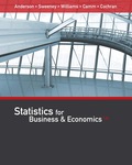
Thus, the chi-square test statistic is 77.74.

Degrees of freedom:

The degrees of freedom are $df=\left(r-1\right)\left(c-1\right)$ for the contingency table of r rows and c columns.

In the given problem $r=5$ and $c=4$.

Therefore,

$\begin{array}{c}df=\left(5-1\right)\left(4-1\right)\\ =12\end{array}$

Level of significance:

The given level of significance is $\alpha =0.05$.

p-value:

Software procedure:

Step -by-step software procedure to obtain p-value using MINITAB software is as follows:

• Select Graph > Probability distribution plot > view probability
• Select chi-square under distribution and enter 12 in degrees of freedom.
• Choose X-Value and Right Tail for the region of the curve to shade.
• Enter the X-value as 77.74 under shaded area.
• Select OK.
• Output using MINITAB software is given below:

From the MINITAB output, the p-value is 0.

Rejection rule:

If the $p\text{-value}\le \alpha$, then reject the null hypothesis.

Conclusion:

Here, the p-value is less than the level of significance.

That is, $p\text{-value}\left(=0\right)<\alpha \left(=0.05\right)$

Thus, the decision is “reject the null hypothesis”.

Therefore, the data provide sufficient evidence to conclude that column variable is not independent of row variable. That is, there is an association between column and row variable.

Thus, the data provide sufficient evidence to conclude that people’s attitude toward the actress who was most deserving of the 2013 Academy Award for Actress in a Leading Role is not independent of respondent age.