
Concept explainers
Videos
The appraisal of a warehouse can appear straightforward compared to other appraisal assignments. A warehouse appraisal involves comparing a building that is primarily an open shell to other such buildings. However, there are still a number of warehouse attributes that are plausibly related to appraised value. The article “Challenges in Appraising ‘Simple’ Warehouse Properties” (Donald Sonneman, The Appraisal Journal, April 2001, 174–178) gives the accompanying data on truss height (ft), which determines how high stored goods can be stacked, and sale price ($) per square foot.
| Height | 12 | 14 | 14 | 15 | 15 | 16 | 18 | 22 | 22 | 24 |
| Price | 35.53 | 37.82 | 36.90 | 40.00 | 38.00 | 37.50 | 41.00 | 48.50 | 47.00 | 47.50 |
| Height | 24 | 26 | 26 | 27 | 28 | 30 | 30 | 33 | 36 |
| Price | 46.20 | 50.35 | 49.13 | 48.07 | 50.90 | 54.78 | 54.32 | 57.17 | 57.45 |
- a. Is it the case that truss height and sale price are “deter-ministically” related—i.e., that sale price is determined completely and uniquely by truss height? [Hint: Look at the data.]
- b. Construct a
scatterplot of the data. What does it suggest? - c. Determine the equation of the least squares line.
- d. Give a point prediction of price when truss height is 27 ft, and calculate the corresponding residual.
- e. What percentage of observed variation in sale price can be attributed to the approximate linear relationship between truss height and price?
a.
Explain whether the variable sale price is completely and uniquely determined by height.
Answer to Problem 68SE
No, the sale price is not uniquely determined by height.
Explanation of Solution
Given info:
The data represents the values of the variables height in feet and price in dollars of the stored goods.
Justification:
Uniquely determined:
Uniquely determined in the sense, for each value of the height, the sale price should be unique. That is, all the equal heights should be associated with same sale price and all the unequal heights should be associated with different sale price values.
From the dataset, it is observed that the equal heights also results in different sale price.
That is, the height value 14 is repeated twice with two different sale price values.
Hence, it can be concluded that sale price is not uniquely determined by height.
b.
Draw a scatterplot of the variables height and sale price.
Answer to Problem 68SE
Output using MINITAB software is given below:
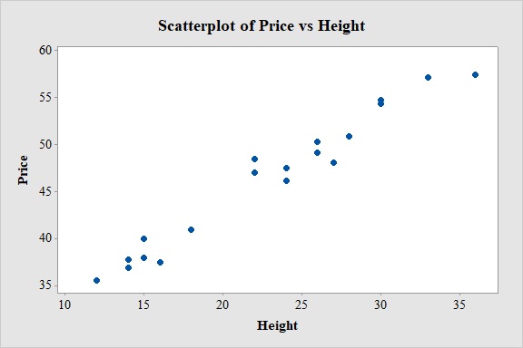
The association between the variables height and sale price is positive, strong and linear.
Explanation of Solution
Justification:
Software Procedure:
Step by step procedure to obtain scatterplot using Minitab software is given as,
- Choose Graph > Scatter plot.
- Choose Simple, and then click OK.
- Under Y variables, enter a column of Price.
- Under X variables, enter a column of Height.
- Click Ok.
Associated variables:
Two variables are associated or related if the value of one variable gives you information about the value of the other variable.
The two variables height and sale price are associated variables.
Direction of association:
If the increase in the values of one variable increases the values of another variable, then the direction is positive. If the increase in the values of one variable decreases the values of another variable, then the direction is negative.
Here, the value of sale price increases with the increase in the value of height.
Hence, the direction of the association is positive.
Form of the association between variable:
The form of the association describes whether the data points follow a linear pattern or some other complicated curves. For data if it appears that a line would do a reasonable job of summarizing the overall pattern in the data. Then, the association between two variables is linear.
From the scatterplot, it is observed that the pattern of the relationship between the variables height and sale price produces a relatively straight line.
Hence the form of the association between the variables height and sale price is linear.
Strength of the association:
The association is said to be strong if all the points are close to the straight line. It is said to be weak if all points are far away from the straight line and it is said to be moderate if the data points are moderately close to straight line.
From the scatterplot, it is observed that the variables will have perfect correlation between them.
Hence, the association between the variables is strong.
Observation:
From the scatterplot it is clear that, as the values of height increases the sale price of the stored goods also increases linearly. Thus, there is a positive association between the variables height and sale price.
c.
Find the regression line for the variables sale price
Answer to Problem 68SE
The regression line for the variables sale price
Explanation of Solution
Calculation:
Linear regression model:
In a linear regression model
Regression:
Software procedure:
Step by step procedure to obtain regression equation using MINITAB software is given as,
- Choose Stat > Regression > Fit Regression Line.
- In Response (Y), enter the column of Price.
- In Predictor (X), enter the column of Height.
- Click OK.
Output using MINITAB software is given below:
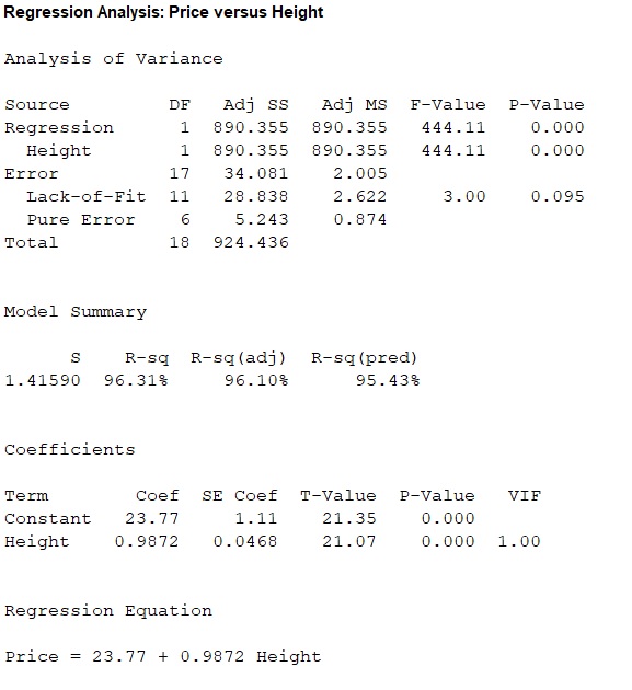
Thus, the regression line for the variables sale price
d.
Find the predicted value of sale price when the height is 27 feet.
Find the corresponding residual of the obtained point prediction.
Answer to Problem 68SE
The predicted value of sale price for 27 feet height stored goods is 50.4244.
The residual of the predicted value of sale price for 27 feet height stored goods is -2.3544.
Explanation of Solution
Calculation:
In a linear regression model
Here, the regression equation is
Point prediction of sale price when the height is 27 feet:
The predicted value of sale price for 27 ft height stored goods is obtained as follows:
Thus, the predicted value of sale price for 27 ft height stored goods is 50.4244.
Residual:
The residual is defined as
If the observed value is less than predicted value then the residual will be negative and if the observed value is greater than predicted value then the residual will be positive.
Residual of predicted value of sale price when the height is 27ft:
The predicted value of sale price for 27 feet height stored goods is 50.4244.
From the given data, the observed value of sale price corresponding to height 27ft is 48.07.
The general formula to obtain residuals is,
Here, the residual values are obtained as follows:
Thus, for a height of 27, the observed sale price is 48.07 and the predicted sale price is 50.4244.
Therefore, the residual is,
Hence, the residual is negative and the predicted sale price 50.4244 is higher than the actual sale price for a height of 27 ft.
Hence, it is preferable to have negative residual.
e.
Find the proportion of observed variation in sale price that can be explained by the obtained regression model.
Answer to Problem 68SE
The proportion of observed variation in sale price that can be explained by the obtained regression model is 96.31%.
Explanation of Solution
Justification:
The coefficient of determination (
The general formula to obtain coefficient of variation is,
From the regression output obtained in part (a), the value of coefficient of determination is 0.631.
Thus, the coefficient of determination is
The coefficient of determination describes the amount of variation in the observed values of the response variable that is explained by the regression.
Interpretation:
From this coefficient of determination it can be said that, the height can explain only 96.31% variability in sale price. Then remaining variability of sale price is explained by other variables.
Thus, the percentage of variation in the observed values of sale price that is explained by the regression is 96.31%, which indicates that 96.31% of the variability in sale price is explained by variability in the height using the linear regression model.
Want to see more full solutions like this?
Chapter 12 Solutions
Probability and Statistics for Engineering and the Sciences


- You have been hired as an intern to run analyses on the data and report the results back to Sarah; the five questions that Sarah needs you to address are given below. Does there appear to be a positive or negative relationship between price and screen size? Use a scatter plot to examine the relationship. Determine and interpret the correlation coefficient between the two variables. In your interpretation, discuss the direction of the relationship (positive, negative, or zero relationship). Also discuss the strength of the relationship. Estimate the relationship between screen size and price using a simple linear regression model and interpret the estimated coefficients. (In your interpretation, tell the dollar amount by which price will change for each unit of increase in screen size). Include the manufacturer dummy variable (Samsung=1, 0 otherwise) and estimate the relationship between screen size, price and manufacturer dummy as a multiple linear regression model. Interpret the…arrow_forwardDoes there appear to be a positive or negative relationship between price and screen size? Use a scatter plot to examine the relationship. How to take snapshots: if you use a MacBook, press Command+ Shift+4 to take snapshots. If you are using Windows, use the Snipping Tool to take snapshots. Question 1: Determine and interpret the correlation coefficient between the two variables. In your interpretation, discuss the direction of the relationship (positive, negative, or zero relationship). Also discuss the strength of the relationship. Value of correlation coefficient: Direction of the relationship (positive, negative, or zero relationship): Strength of the relationship (strong/moderate/weak): Question 2: Estimate the relationship between screen size and price using a simple linear regression model and interpret the estimated coefficients. In your interpretation, tell the dollar amount by which price will change for each unit of increase in screen size. (The answer for the…arrow_forwardIn this problem, we consider a Brownian motion (W+) t≥0. We consider a stock model (St)t>0 given (under the measure P) by d.St 0.03 St dt + 0.2 St dwt, with So 2. We assume that the interest rate is r = 0.06. The purpose of this problem is to price an option on this stock (which we name cubic put). This option is European-type, with maturity 3 months (i.e. T = 0.25 years), and payoff given by F = (8-5)+ (a) Write the Stochastic Differential Equation satisfied by (St) under the risk-neutral measure Q. (You don't need to prove it, simply give the answer.) (b) Give the price of a regular European put on (St) with maturity 3 months and strike K = 2. (c) Let X = S. Find the Stochastic Differential Equation satisfied by the process (Xt) under the measure Q. (d) Find an explicit expression for X₁ = S3 under measure Q. (e) Using the results above, find the price of the cubic put option mentioned above. (f) Is the price in (e) the same as in question (b)? (Explain why.)arrow_forward
- Problem 4. Margrabe formula and the Greeks (20 pts) In the homework, we determined the Margrabe formula for the price of an option allowing you to swap an x-stock for a y-stock at time T. For stocks with initial values xo, yo, common volatility σ and correlation p, the formula was given by Fo=yo (d+)-x0Þ(d_), where In (±² Ꭲ d+ õ√T and σ = σ√√√2(1 - p). дго (a) We want to determine a "Greek" for ỡ on the option: find a formula for θα (b) Is дго θα positive or negative? (c) We consider a situation in which the correlation p between the two stocks increases: what can you say about the price Fo? (d) Assume that yo< xo and p = 1. What is the price of the option?arrow_forwardWe consider a 4-dimensional stock price model given (under P) by dẴ₁ = µ· Xt dt + йt · ΣdŴt where (W) is an n-dimensional Brownian motion, π = (0.02, 0.01, -0.02, 0.05), 0.2 0 0 0 0.3 0.4 0 0 Σ= -0.1 -4a За 0 0.2 0.4 -0.1 0.2) and a E R. We assume that ☑0 = (1, 1, 1, 1) and that the interest rate on the market is r = 0.02. (a) Give a condition on a that would make stock #3 be the one with largest volatility. (b) Find the diversification coefficient for this portfolio as a function of a. (c) Determine the maximum diversification coefficient d that you could reach by varying the value of a? 2arrow_forwardQuestion 1. Your manager asks you to explain why the Black-Scholes model may be inappro- priate for pricing options in practice. Give one reason that would substantiate this claim? Question 2. We consider stock #1 and stock #2 in the model of Problem 2. Your manager asks you to pick only one of them to invest in based on the model provided. Which one do you choose and why ? Question 3. Let (St) to be an asset modeled by the Black-Scholes SDE. Let Ft be the price at time t of a European put with maturity T and strike price K. Then, the discounted option price process (ert Ft) t20 is a martingale. True or False? (Explain your answer.) Question 4. You are considering pricing an American put option using a Black-Scholes model for the underlying stock. An explicit formula for the price doesn't exist. In just a few words (no more than 2 sentences), explain how you would proceed to price it. Question 5. We model a short rate with a Ho-Lee model drt = ln(1+t) dt +2dWt. Then the interest rate…arrow_forward
- In this problem, we consider a Brownian motion (W+) t≥0. We consider a stock model (St)t>0 given (under the measure P) by d.St 0.03 St dt + 0.2 St dwt, with So 2. We assume that the interest rate is r = 0.06. The purpose of this problem is to price an option on this stock (which we name cubic put). This option is European-type, with maturity 3 months (i.e. T = 0.25 years), and payoff given by F = (8-5)+ (a) Write the Stochastic Differential Equation satisfied by (St) under the risk-neutral measure Q. (You don't need to prove it, simply give the answer.) (b) Give the price of a regular European put on (St) with maturity 3 months and strike K = 2. (c) Let X = S. Find the Stochastic Differential Equation satisfied by the process (Xt) under the measure Q. (d) Find an explicit expression for X₁ = S3 under measure Q. (e) Using the results above, find the price of the cubic put option mentioned above. (f) Is the price in (e) the same as in question (b)? (Explain why.)arrow_forwardThe managing director of a consulting group has the accompanying monthly data on total overhead costs and professional labor hours to bill to clients. Complete parts a through c. Question content area bottom Part 1 a. Develop a simple linear regression model between billable hours and overhead costs. Overhead Costsequals=212495.2212495.2plus+left parenthesis 42.4857 right parenthesis42.485742.4857times×Billable Hours (Round the constant to one decimal place as needed. Round the coefficient to four decimal places as needed. Do not include the $ symbol in your answers.) Part 2 b. Interpret the coefficients of your regression model. Specifically, what does the fixed component of the model mean to the consulting firm? Interpret the fixed term, b 0b0, if appropriate. Choose the correct answer below. A. The value of b 0b0 is the predicted billable hours for an overhead cost of 0 dollars. B. It is not appropriate to interpret b 0b0, because its value…arrow_forwardUsing the accompanying Home Market Value data and associated regression line, Market ValueMarket Valueequals=$28,416+$37.066×Square Feet, compute the errors associated with each observation using the formula e Subscript ieiequals=Upper Y Subscript iYiminus−ModifyingAbove Upper Y with caret Subscript iYi and construct a frequency distribution and histogram. LOADING... Click the icon to view the Home Market Value data. Question content area bottom Part 1 Construct a frequency distribution of the errors, e Subscript iei. (Type whole numbers.) Error Frequency minus−15 comma 00015,000less than< e Subscript iei less than or equals≤minus−10 comma 00010,000 0 minus−10 comma 00010,000less than< e Subscript iei less than or equals≤minus−50005000 5 minus−50005000less than< e Subscript iei less than or equals≤0 21 0less than< e Subscript iei less than or equals≤50005000 9…arrow_forward
- The managing director of a consulting group has the accompanying monthly data on total overhead costs and professional labor hours to bill to clients. Complete parts a through c Overhead Costs Billable Hours345000 3000385000 4000410000 5000462000 6000530000 7000545000 8000arrow_forwardUsing the accompanying Home Market Value data and associated regression line, Market ValueMarket Valueequals=$28,416plus+$37.066×Square Feet, compute the errors associated with each observation using the formula e Subscript ieiequals=Upper Y Subscript iYiminus−ModifyingAbove Upper Y with caret Subscript iYi and construct a frequency distribution and histogram. Square Feet Market Value1813 911001916 1043001842 934001814 909001836 1020002030 1085001731 877001852 960001793 893001665 884001852 1009001619 967001690 876002370 1139002373 1131001666 875002122 1161001619 946001729 863001667 871001522 833001484 798001589 814001600 871001484 825001483 787001522 877001703 942001485 820001468 881001519 882001518 885001483 765001522 844001668 909001587 810001782 912001483 812001519 1007001522 872001684 966001581 86200arrow_forwarda. Find the value of A.b. Find pX(x) and py(y).c. Find pX|y(x|y) and py|X(y|x)d. Are x and y independent? Why or why not?arrow_forward
 Glencoe Algebra 1, Student Edition, 9780079039897...AlgebraISBN:9780079039897Author:CarterPublisher:McGraw Hill
 Big Ideas Math A Bridge To Success Algebra 1: Stu...AlgebraISBN:9781680331141Author:HOUGHTON MIFFLIN HARCOURTPublisher:Houghton Mifflin Harcourt
 Holt Mcdougal Larson Pre-algebra: Student Edition...AlgebraISBN:9780547587776Author:HOLT MCDOUGALPublisher:HOLT MCDOUGAL
 Functions and Change: A Modeling Approach to Coll...AlgebraISBN:9781337111348Author:Bruce Crauder, Benny Evans, Alan NoellPublisher:Cengage Learning