
Concept explainers
Videos
a.
Find whether there is a difference in the variation in team salary among the people from Country A and National league teams.
a.
Answer to Problem 50DE
There is no difference in the variance in team salary among the people from Country A and National league teams.
Explanation of Solution
The null and alternative hypotheses are stated below:
Null hypothesis: There is no difference in the variance in team salary among Country A and National league teams.
Alternative hypothesis: There is difference in the variance in team salary among Country A and National league teams.
Step-by-step procedure to obtain the test statistic using Excel:
- In the first column, enter the salaries of Country A’s team.
- In the second column, enter the salaries of National team.
- Select the Data tab on the top menu.
- Select Data Analysis and Click on: F-Test, Two-sample for variances and then click on OK.
- In the dialog box, select Input
Range . - Click OK
Output obtained using Excel is represented as follows:
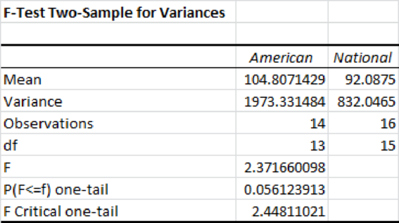
From the above output, the F- test statistic value is 2.37 and its p-value is 0.056.
Decision Rule:
If the p-value is less than the level of significance, reject the null hypothesis. Otherwise, fail to reject the null hypothesis.
Conclusion:
The significance level is 0.05. The p-value is 0.056 and it is greater than the significance level. The null hypothesis is rejected at the 0.05 significance level.
Thus, there is no difference in the variance in team salary among Country A and National league teams.
b.
Create a variable that classifies a team’s total attendance into three groups.
Find whether there is a difference in the
b.
Answer to Problem 50DE
There is no difference in the mean number of games won among the three groups.
Explanation of Solution
Let X represent the total attendance into three groups. Samples 1, 2, and 3 are “less than 2 (million)”, 2 up to 3, and 3 or more attendance of teams of three groups, respectively.
The following table gives the number of games won by the three groups of attendances.
| Sample 1 | Sample 2 | Sample 3 |
| 85 | 81 | 69 |
| 68 | 94 | 88 |
| 55 | 93 | 89 |
| 72 | 61 | 86 |
| 94 | 97 | 74 |
| 75 | 64 | 81 |
| 69 | 94 | |
| 83 | 88 | |
| 66 | 93 | |
| 95 | ||
| 79 | ||
| 76 | ||
| 73 | ||
| 98 |
The null and alternative hypotheses are as follows:
Null hypothesis: There is no difference in the mean number of games won among the three groups.
Alternative hypothesis: There is a difference in the mean number of games won among the three groups
Step-by-step procedure to obtain the test statistic using Excel:
- In Sample 1, enter the number of games won by the team, which is less than 2 million attendances.
- In Sample 2, enter the number of games won by the team of 2 up to 3 million attendances.
- In Sample 3, enter the number of games won by the team of 3 or more million attendances.
- Select the Data tab on the top menu.
- Select Data Analysis and Click on: ANOVA: Single factor and then click on OK.
- In the dialog box, select Input Range.
- Click OK
Output obtained using Excel is represented as follows:
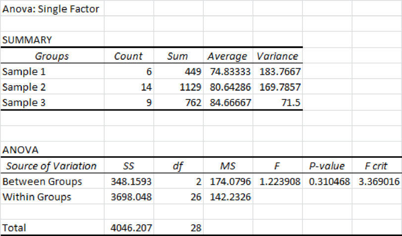
From the above output, the F test statistic value is 1.22 and the p-value is 0.31.
Conclusion:
The level of significance is 0.05. The p-value is greater than the significance level. Hence, one can fail to reject the null hypothesis at the 0.05 significance level. Thus, there is no difference in the mean number of games won among the three groups.
c.
Find whether there is a difference in the mean number of home runs hit per team using the variable defined in Part b.
c.
Answer to Problem 50DE
There is no difference in the mean number of home runs hit per team.
Explanation of Solution
The null and alternative hypotheses are stated below:
Null hypothesis: There is no difference in the mean number of home runs hit per team.
Alternative hypothesis: There is a difference in the mean number of home runs hit per team.
The following table gives the number of home runs per each team, which is defined in Part b.
| Sample 1 | Sample 2 | Sample 3 |
| 211 | 165 | 165 |
| 136 | 149 | 163 |
| 146 | 214 | 187 |
| 131 | 137 | 116 |
| 195 | 172 | 245 |
| 149 | 166 | 158 |
| 175 | 137 | 103 |
| 202 | 159 | |
| 131 | 200 | |
| 139 | ||
| 170 | ||
| 121 | ||
| 198 | ||
| 194 |
Step-by-step procedure to obtain the test statistic using Excel:
- In Sample 1, enter the number of home runs hit by the group of less than 2 million attendances.
- In Sample 2, enter the number of home runs hit by the group of 2 up to 3 million attendances.
- In Sample 3, enter the number of home runs hit by the group of 3 or more million attendances.
- Select the Data tab on the top menu.
- Select Data Analysis and Click on: ANOVA: Single factor and then click on OK.
- In the dialog box, select Input Range.
- Click OK
Output obtained using Excel is represented as follows:
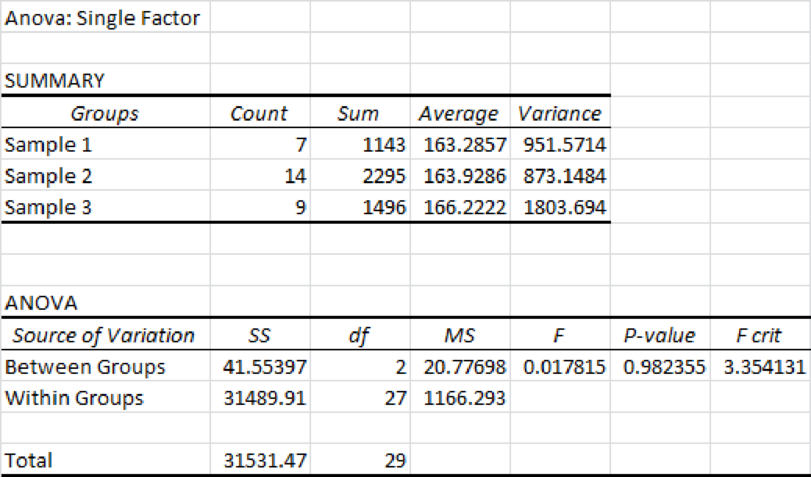
From the above output, the F test statistic value is 0.018 and the p-value is 0.9823.
Conclusion:
The level of significance is 0.05 and the p-value is greater than the significance level. Hence, one fails to reject the null hypothesis at the 0.05 significance level. Thus, there is no difference in the mean number of home runs hit per team.
d.
Find whether there is a difference in the mean salary of the three groups.
d.
Answer to Problem 50DE
The mean salaries are different for each group.
Explanation of Solution
The null and alternative hypotheses are stated below:
Null hypothesis: The mean salary of the three groups is equal.
Alternative hypothesis: At least one mean salary is different from other.
The following table provides the salary of each group that is defined in Part b.
| Sample 1 | Sample 2 | Sample 3 |
| 96.9 | 74.3 | 173.2 |
| 78.4 | 83.3 | 132.3 |
| 60.7 | 81.4 | 154.5 |
| 60.9 | 88.2 | 95.1 |
| 55.4 | 82.2 | 198 |
| 82 | 78.1 | 174.5 |
| 64.2 | 118.1 | 117.6 |
| 97.7 | 110.3 | |
| 94.1 | 120.5 | |
| 93.4 | ||
| 63.4 | ||
| 55.2 | ||
| 75.5 | ||
| 81.3 |
Step-by-step procedure to obtain the test statistic using Excel:
- In Sample 1, enter the salary of the group of less than 2 million attendances.
- In Sample 2, enter the salary of the group of 2 up to 3 million attendances.
- In Sample 3, enter the salary of the group of 3 or more million attendances.
- Select the Data tab on the top menu.
- Select Data Analysis and Click on: ANOVA: Single factor and then click on OK.
- In the dialog box, select Input Range.
- Click OK
Output obtained using Excel is represented as follows:
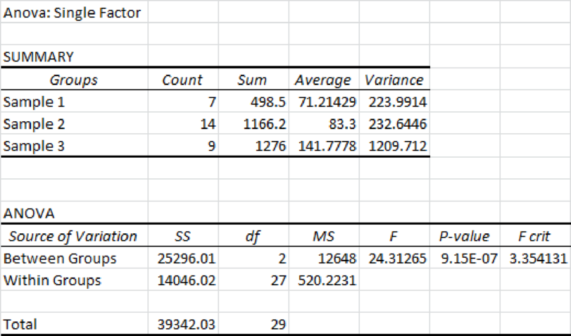
From the above output, the F test statistic value is 24.31 and the p-value is 0.
Conclusion:
The level of significance is 0.05 and the p-value is less than the significance level. Hence, one can reject the null hypothesis at the 0.05 significance level. Thus, the mean salaries are different for each group.
Want to see more full solutions like this?
Chapter 12 Solutions
Statistical Techniques in Business and Economics


- Question 1. Your manager asks you to explain why the Black-Scholes model may be inappro- priate for pricing options in practice. Give one reason that would substantiate this claim? Question 2. We consider stock #1 and stock #2 in the model of Problem 2. Your manager asks you to pick only one of them to invest in based on the model provided. Which one do you choose and why ? Question 3. Let (St) to be an asset modeled by the Black-Scholes SDE. Let Ft be the price at time t of a European put with maturity T and strike price K. Then, the discounted option price process (ert Ft) t20 is a martingale. True or False? (Explain your answer.) Question 4. You are considering pricing an American put option using a Black-Scholes model for the underlying stock. An explicit formula for the price doesn't exist. In just a few words (no more than 2 sentences), explain how you would proceed to price it. Question 5. We model a short rate with a Ho-Lee model drt = ln(1+t) dt +2dWt. Then the interest rate…arrow_forwardIn this problem, we consider a Brownian motion (W+) t≥0. We consider a stock model (St)t>0 given (under the measure P) by d.St 0.03 St dt + 0.2 St dwt, with So 2. We assume that the interest rate is r = 0.06. The purpose of this problem is to price an option on this stock (which we name cubic put). This option is European-type, with maturity 3 months (i.e. T = 0.25 years), and payoff given by F = (8-5)+ (a) Write the Stochastic Differential Equation satisfied by (St) under the risk-neutral measure Q. (You don't need to prove it, simply give the answer.) (b) Give the price of a regular European put on (St) with maturity 3 months and strike K = 2. (c) Let X = S. Find the Stochastic Differential Equation satisfied by the process (Xt) under the measure Q. (d) Find an explicit expression for X₁ = S3 under measure Q. (e) Using the results above, find the price of the cubic put option mentioned above. (f) Is the price in (e) the same as in question (b)? (Explain why.)arrow_forwardThe managing director of a consulting group has the accompanying monthly data on total overhead costs and professional labor hours to bill to clients. Complete parts a through c. Question content area bottom Part 1 a. Develop a simple linear regression model between billable hours and overhead costs. Overhead Costsequals=212495.2212495.2plus+left parenthesis 42.4857 right parenthesis42.485742.4857times×Billable Hours (Round the constant to one decimal place as needed. Round the coefficient to four decimal places as needed. Do not include the $ symbol in your answers.) Part 2 b. Interpret the coefficients of your regression model. Specifically, what does the fixed component of the model mean to the consulting firm? Interpret the fixed term, b 0b0, if appropriate. Choose the correct answer below. A. The value of b 0b0 is the predicted billable hours for an overhead cost of 0 dollars. B. It is not appropriate to interpret b 0b0, because its value…arrow_forward
- Using the accompanying Home Market Value data and associated regression line, Market ValueMarket Valueequals=$28,416+$37.066×Square Feet, compute the errors associated with each observation using the formula e Subscript ieiequals=Upper Y Subscript iYiminus−ModifyingAbove Upper Y with caret Subscript iYi and construct a frequency distribution and histogram. LOADING... Click the icon to view the Home Market Value data. Question content area bottom Part 1 Construct a frequency distribution of the errors, e Subscript iei. (Type whole numbers.) Error Frequency minus−15 comma 00015,000less than< e Subscript iei less than or equals≤minus−10 comma 00010,000 0 minus−10 comma 00010,000less than< e Subscript iei less than or equals≤minus−50005000 5 minus−50005000less than< e Subscript iei less than or equals≤0 21 0less than< e Subscript iei less than or equals≤50005000 9…arrow_forwardThe managing director of a consulting group has the accompanying monthly data on total overhead costs and professional labor hours to bill to clients. Complete parts a through c Overhead Costs Billable Hours345000 3000385000 4000410000 5000462000 6000530000 7000545000 8000arrow_forwardUsing the accompanying Home Market Value data and associated regression line, Market ValueMarket Valueequals=$28,416plus+$37.066×Square Feet, compute the errors associated with each observation using the formula e Subscript ieiequals=Upper Y Subscript iYiminus−ModifyingAbove Upper Y with caret Subscript iYi and construct a frequency distribution and histogram. Square Feet Market Value1813 911001916 1043001842 934001814 909001836 1020002030 1085001731 877001852 960001793 893001665 884001852 1009001619 967001690 876002370 1139002373 1131001666 875002122 1161001619 946001729 863001667 871001522 833001484 798001589 814001600 871001484 825001483 787001522 877001703 942001485 820001468 881001519 882001518 885001483 765001522 844001668 909001587 810001782 912001483 812001519 1007001522 872001684 966001581 86200arrow_forward
- For a binary asymmetric channel with Py|X(0|1) = 0.1 and Py|X(1|0) = 0.2; PX(0) = 0.4 isthe probability of a bit of “0” being transmitted. X is the transmitted digit, and Y is the received digit.a. Find the values of Py(0) and Py(1).b. What is the probability that only 0s will be received for a sequence of 10 digits transmitted?c. What is the probability that 8 1s and 2 0s will be received for the same sequence of 10 digits?d. What is the probability that at least 5 0s will be received for the same sequence of 10 digits?arrow_forwardV2 360 Step down + I₁ = I2 10KVA 120V 10KVA 1₂ = 360-120 or 2nd Ratio's V₂ m 120 Ratio= 360 √2 H I2 I, + I2 120arrow_forwardQ2. [20 points] An amplitude X of a Gaussian signal x(t) has a mean value of 2 and an RMS value of √(10), i.e. square root of 10. Determine the PDF of x(t).arrow_forward
 Big Ideas Math A Bridge To Success Algebra 1: Stu...AlgebraISBN:9781680331141Author:HOUGHTON MIFFLIN HARCOURTPublisher:Houghton Mifflin Harcourt
 Glencoe Algebra 1, Student Edition, 9780079039897...AlgebraISBN:9780079039897Author:CarterPublisher:McGraw Hill
 Holt Mcdougal Larson Pre-algebra: Student Edition...AlgebraISBN:9780547587776Author:HOLT MCDOUGALPublisher:HOLT MCDOUGAL