
Videos
To test: the null hypothesis and show that it is rejected at the
Explanation of Solution
Given information :
Concept Involved:
In order to decide whether the presumed hypothesis for data sample stands accurate for the entire population or not we use the hypothesis testing.
The critical value from Table A.4, using degrees of freedom of
The values of two qualitative variables are connected and denoted in a contingency table.
This table consists of rows and column. The variables in each row and each column of the table represent a category. The number of rows of contingency table is represented by letter ‘r’ and number of column of contingency table is represented by letter ‘c’.
The formula to find the number of degree of freedom of contingency table is
Calculation:
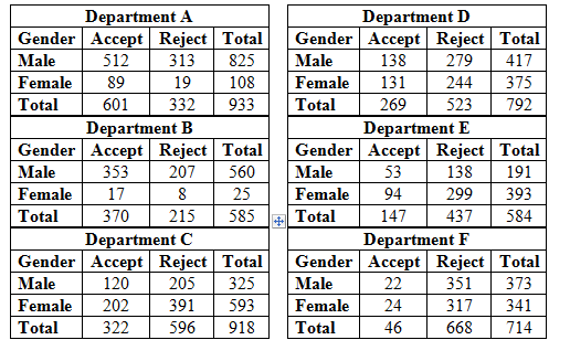
For department A:
| Department A | |||
| Gender | Accept | Reject | Total |
| Male | 512 | 313 | 825 |
| Female | 89 | 19 | 108 |
| Total | 601 | 332 | 933 |
| Finding the expected frequency for the cell corresponding to: | The expected frequency |
| Number of male applicants acceptedin department A The row total is 825, the column total is 601, and the grand total is 933. | |
| Number of male applicants rejectedin department A The row total is 825, the column total is 332, and the grand total is 933. | |
| Number of female applicantsaccepted in department A The row total is 108, the column total is 601, and the grand total is 933. | |
| Number of female applicantsrejected in department A The row total is 108, the column total is 332, and the grand total is 933. |
| Finding the value of the chi-square corresponding to: | |
| Number of male applicants acceptedin department A The observed frequency is 512 and expected frequency is 531.43 | |
| Number of male applicants rejectedin department A The observed frequency is 313 and expected frequency is 293.57 | |
| Number of female applicantsaccepted in department A The observed frequency is 89 and expected frequency is 69.57 | |
| Number of female applicantsrejected in department A The observed frequency is 19 and expected frequency is 38.43 |
To compute the test statistics, we use the observed frequencies and expected frequency:
In department A, % of male accepted =
For department B:
| Department B | |||
| Gender | Accept | Reject | Total |
| Male | 353 | 207 | 560 |
| Female | 17 | 8 | 25 |
| Total | 370 | 215 | 585 |
| Finding the expected frequency for the cell corresponding to: | The expected frequency |
| Number of male applicants acceptedin department B The row total is 560, the column total is 370, and the grand total is 585. | |
| Number of male applicants rejectedin department B The row total is 560, the column total is 215, and the grand total is 585. | |
| Number of female applicantsaccepted in department B The row total is 25, the column total is 370, and the grand total is 585. | |
| Number of female applicantsrejected in department B The row total is 25, the column total is 215, and the grand total is 585. |
| Finding the value of the chi-square corresponding to: | |
| Number of male applicants acceptedin department B The observed frequency is 353 and expected frequency is 354.19 | |
| Number of male applicants rejectedin department B The observed frequency is 207 and expected frequency is 205.81 | |
| Number of female applicantsaccepted in department B The observed frequency is 17 and expected frequency is 15.81 | |
| Number of female applicantsrejected in department B The observed frequency is 8 and expected frequency is 9.19 |
To compute the test statistics, we use the observed frequencies and expected frequency:
In department B, % of male accepted =
For department C:
| Department C | |||
| Gender | Accept | Reject | Total |
| Male | 120 | 205 | 325 |
| Female | 202 | 391 | 593 |
| Total | 322 | 596 | 918 |
| Finding the expected frequency for the cell corresponding to: | The expected frequency |
| Number of male applicants acceptedin department C The row total is 325, the column total is 322, and the grand total is 918. | |
| Number of male applicants rejectedin department C The row total is 325, the column total is 596, and the grand total is918. | |
| Number of female applicantsaccepted in department C The row total is 593, the column total is 322, and the grand total is 918. | |
| Number of female applicantsrejected in department C The row total is 593, the column total is 596, and the grand total is 918. |
| Finding the value of the chi-square corresponding to: | |
| Number of male applicants acceptedin department C The observed frequency is 120 and expected frequency is 114 | |
| Number of male applicants rejectedin department C The observed frequency is 205 and expected frequency is 211 | |
| Number of female applicantsaccepted in department C The observed frequency is 202 and expected frequency is 208 | |
| Number of female applicantsrejected in department C The observed frequency is 391 and expected frequency is 385 |
To compute the test statistics, we use the observed frequencies and expected frequency:
In department C, % of male accepted =
For department D:
| Department D | |||
| Gender | Accept | Reject | Total |
| Male | 138 | 279 | 417 |
| Female | 131 | 244 | 375 |
| Total | 269 | 523 | 792 |
| Finding the expected frequency for the cell corresponding to: | The expected frequency |
| Number of male applicants acceptedin department D The row total is 417, the column total is 269, and the grand total is 792. | |
| Number of male applicants rejectedin department D The row total is 417, the column total is 523, and the grand total is792. | |
| Number of female applicantsaccepted in department D The row total is 375, the column total is 269, and the grand total is 792. | |
| Number of female applicantsrejected in department D The row total is 375, the column total is 523, and the grand total is 792. |
| Finding the value of the chi-square corresponding to: | |
| Number of male applicants acceptedin department D The observed frequency is 138 and expected frequency is 141.63 | |
| Number of male applicants rejectedin department D The observed frequency is 279 and expected frequency is 275.37 | |
| Number of female applicantsaccepted in department D The observed frequency is 131 and expected frequency is 127.37 | |
| Number of female applicantsrejected in department D The observed frequency is 244 and expected frequency is 247.63 |
To compute the test statistics, we use the observed frequencies and expected frequency:
In department D, % of male accepted =
For department E:
| Department E | |||
| Gender | Accept | Reject | Total |
| Male | 53 | 138 | 191 |
| Female | 94 | 299 | 393 |
| Total | 147 | 437 | 584 |
| Finding the expected frequency for the cell corresponding to: | The expected frequency |
| Number of male applicants acceptedin department E The row total is 191, the column total is 147, and the grand total is 584. | |
| Number of male applicants rejectedin department E The row total is 191, the column total is 437, and the grand total is584. | |
| Number of female applicantsaccepted in department E The row total is 393, the column total is 147, and the grand total is 584. | |
| Number of female applicantsrejected in department E The row total is 393, the column total is 437, and the grand total is 584. |
| Finding the value of the chi-square corresponding to: | |
| Number of male applicants acceptedin department E The observed frequency is 53 and expected frequency is 48.08 | |
| Number of male applicants rejectedin department E The observed frequency is 138 and expected frequency is 142.92 | |
| Number of female applicantsaccepted in department E The observed frequency is 94 and expected frequency is 98.92 | |
| Number of female applicantsrejected in department E The observed frequency is 299 and expected frequency is 294.08 |
To compute the test statistics, we use the observed frequencies and expected frequency:
In department E, % of male accepted =
For department F:
| Department F | |||
| Gender | Accept | Reject | Total |
| Male | 22 | 351 | 373 |
| Female | 24 | 317 | 341 |
| Total | 46 | 668 | 714 |
| Finding the expected frequency for the cell corresponding to: | The expected frequency |
| Number of male applicants acceptedin department F The row total is 373, the column total is 46, and the grand total is 714. | |
| Number of male applicants rejectedin department F The row total is 373, the column total is 668, and the grand total is714. | |
| Number of female applicantsaccepted in department F The row total is 341, the column total is 46, and the grand total is 714. | |
| Number of female applicantsrejected in department F The row total is 341, the column total is 668, and the grand total is 714. |
| Finding the value of the chi-square corresponding to: | |
| Number of male applicants acceptedin department F The observed frequency is 22 and expected frequency is 24.03 | |
| Number of male applicants rejectedin department F The observed frequency is 351 and expected frequency is 348.97 | |
| Number of female applicantsaccepted in department F The observed frequency is 24 and expected frequency is 21.97 | |
| Number of female applicantsrejected in department F The observed frequency is 317 and expected frequency is 319.03 |
To compute the test statistics, we use the observed frequencies and expected frequency:
In department E, % of male accepted =
Here r represents the number of rows and c represents the number of columns.
For all the contingency table
| Degrees of freedom | Table A.4 Critical Values for the chi-square Distribution | |||||||||
| 0.995 | 0.99 | 0.975 | 0.95 | 0.90 | 0.10 | 0.05 | 0.025 | 0.01 | 0.005 | |
| 1 | 0.000 | 0.000 | 0.001 | 0.004 | 0.016 | 2.706 | 3.841 | 5.024 | 6.635 | 7.879 |
| 2 | 0.010 | 0.020 | 0.051 | 0.103 | 0.211 | 4.605 | 5.991 | 7.378 | 9.210 | 10.597 |
| 3 | 0.072 | 0.115 | 0.216 | 0.352 | 0.584 | 6.251 | 7.815 | 9.348 | 11.345 | 12.838 |
| 4 | 0.207 | 0.297 | 0.484 | 0.711 | 1.064 | 7.779 | 9.488 | 11.143 | 13.277 | 14.860 |
| 5 | 0.412 | 0.554 | 0.831 | 1.145 | 1.610 | 9.236 | 11.070 | 12.833 | 15.086 | 16.750 |
The critical value is same for all the contingency table.
Conclusion:
For department A:
Test statistic: 17.25; Critical value: 6.635.
For department B:
Test statistic: 0.25; Critical value: 6.635.
For department C:
Test statistic: 0.75; Critical value: 6.635.
For department D:
Test statistic: 0.30; Critical value: 6.635.
For department E:
Test statistic: 1.00; Critical value: 6.635.
For department F:
Test statistic: 0.39; Critical value: 6.635.
In departmentA, 82.4% of the women were accepted, but only 62.1% of themen were accepted.
Want to see more full solutions like this?
Chapter 12 Solutions
Elementary Statistics 2nd Edition


- Business discussarrow_forwardBusiness discussarrow_forwardI just need to know why this is wrong below: What is the test statistic W? W=5 (incorrect) and What is the p-value of this test? (p-value < 0.001-- incorrect) Use the Wilcoxon signed rank test to test the hypothesis that the median number of pages in the statistics books in the library from which the sample was taken is 400. A sample of 12 statistics books have the following numbers of pages pages 127 217 486 132 397 297 396 327 292 256 358 272 What is the sum of the negative ranks (W-)? 75 What is the sum of the positive ranks (W+)? 5What type of test is this? two tailedWhat is the test statistic W? 5 These are the critical values for a 1-tailed Wilcoxon Signed Rank test for n=12 Alpha Level 0.001 0.005 0.01 0.025 0.05 0.1 0.2 Critical Value 75 70 68 64 60 56 50 What is the p-value for this test? p-value < 0.001arrow_forward
- ons 12. A sociologist hypothesizes that the crime rate is higher in areas with higher poverty rate and lower median income. She col- lects data on the crime rate (crimes per 100,000 residents), the poverty rate (in %), and the median income (in $1,000s) from 41 New England cities. A portion of the regression results is shown in the following table. Standard Coefficients error t stat p-value Intercept -301.62 549.71 -0.55 0.5864 Poverty 53.16 14.22 3.74 0.0006 Income 4.95 8.26 0.60 0.5526 a. b. Are the signs as expected on the slope coefficients? Predict the crime rate in an area with a poverty rate of 20% and a median income of $50,000. 3. Using data from 50 workarrow_forward2. The owner of several used-car dealerships believes that the selling price of a used car can best be predicted using the car's age. He uses data on the recent selling price (in $) and age of 20 used sedans to estimate Price = Po + B₁Age + ε. A portion of the regression results is shown in the accompanying table. Standard Coefficients Intercept 21187.94 Error 733.42 t Stat p-value 28.89 1.56E-16 Age -1208.25 128.95 -9.37 2.41E-08 a. What is the estimate for B₁? Interpret this value. b. What is the sample regression equation? C. Predict the selling price of a 5-year-old sedan.arrow_forwardian income of $50,000. erty rate of 13. Using data from 50 workers, a researcher estimates Wage = Bo+B,Education + B₂Experience + B3Age+e, where Wage is the hourly wage rate and Education, Experience, and Age are the years of higher education, the years of experience, and the age of the worker, respectively. A portion of the regression results is shown in the following table. ni ogolloo bash 1 Standard Coefficients error t stat p-value Intercept 7.87 4.09 1.93 0.0603 Education 1.44 0.34 4.24 0.0001 Experience 0.45 0.14 3.16 0.0028 Age -0.01 0.08 -0.14 0.8920 a. Interpret the estimated coefficients for Education and Experience. b. Predict the hourly wage rate for a 30-year-old worker with four years of higher education and three years of experience.arrow_forward
- 1. If a firm spends more on advertising, is it likely to increase sales? Data on annual sales (in $100,000s) and advertising expenditures (in $10,000s) were collected for 20 firms in order to estimate the model Sales = Po + B₁Advertising + ε. A portion of the regression results is shown in the accompanying table. Intercept Advertising Standard Coefficients Error t Stat p-value -7.42 1.46 -5.09 7.66E-05 0.42 0.05 8.70 7.26E-08 a. Interpret the estimated slope coefficient. b. What is the sample regression equation? C. Predict the sales for a firm that spends $500,000 annually on advertising.arrow_forwardCan you help me solve problem 38 with steps im stuck.arrow_forwardHow do the samples hold up to the efficiency test? What percentages of the samples pass or fail the test? What would be the likelihood of having the following specific number of efficiency test failures in the next 300 processors tested? 1 failures, 5 failures, 10 failures and 20 failures.arrow_forward
- The battery temperatures are a major concern for us. Can you analyze and describe the sample data? What are the average and median temperatures? How much variability is there in the temperatures? Is there anything that stands out? Our engineers’ assumption is that the temperature data is normally distributed. If that is the case, what would be the likelihood that the Safety Zone temperature will exceed 5.15 degrees? What is the probability that the Safety Zone temperature will be less than 4.65 degrees? What is the actual percentage of samples that exceed 5.25 degrees or are less than 4.75 degrees? Is the manufacturing process producing units with stable Safety Zone temperatures? Can you check if there are any apparent changes in the temperature pattern? Are there any outliers? A closer look at the Z-scores should help you in this regard.arrow_forwardNeed help pleasearrow_forwardPlease conduct a step by step of these statistical tests on separate sheets of Microsoft Excel. If the calculations in Microsoft Excel are incorrect, the null and alternative hypotheses, as well as the conclusions drawn from them, will be meaningless and will not receive any points. 4. One-Way ANOVA: Analyze the customer satisfaction scores across four different product categories to determine if there is a significant difference in means. (Hints: The null can be about maintaining status-quo or no difference among groups) H0 = H1=arrow_forward
 Big Ideas Math A Bridge To Success Algebra 1: Stu...AlgebraISBN:9781680331141Author:HOUGHTON MIFFLIN HARCOURTPublisher:Houghton Mifflin Harcourt
 Glencoe Algebra 1, Student Edition, 9780079039897...AlgebraISBN:9780079039897Author:CarterPublisher:McGraw Hill
 Functions and Change: A Modeling Approach to Coll...AlgebraISBN:9781337111348Author:Bruce Crauder, Benny Evans, Alan NoellPublisher:Cengage Learning
 Holt Mcdougal Larson Pre-algebra: Student Edition...AlgebraISBN:9780547587776Author:HOLT MCDOUGALPublisher:HOLT MCDOUGAL