
Concept explainers
Videos
To test: The hypothesis that the mean IQs of the various educational levels of the subjects are equal or not.
Answer to Problem 2DA
There is significant difference between the means
Explanation of Solution
Given info:
The databank shows the IQs of the various educational levels of the subjects.
Calculation:
Answers may vary. One of the possible answers is as follows:
Select random samples from the databank. The samples are given below.
| No high school degree | High school degree | College graduate | Graduate degree |
| 103 | 106 | 110 | 121 |
| 101 | 98 | 106 | 129 |
| 103 | 99 | 116 | 126 |
| 100 | 122 | 100 | 128 |
| 116 | 109 | 113 | 131 |
| 103 | 100 | 114 |
The hypotheses are given below:
Null hypothesis:
Alternative hypothesis:
Here, the difference in the mean percentage of voters in different places is tested. Hence, the claim is that,there is a difference in the mean percentage of voters in different places.
The number of samples k is 4, the sample sizes
The degrees of freedom are
Where
Substitute 4 for k in
Substitute 23 for N and 4 for k in
Critical value:
The critical F-value is obtained using the Table H: The F-Distribution with the level of significance
Procedure:
- Locate 19 in the degrees of freedom, denominator row of the Table H.
- Obtain the value in the corresponding degrees of freedom, numerator column below 3.
That is, the critical value is 3.13.
Rejection region:
The null hypothesis would be rejected if
Software procedure:
Step-by-step procedure to obtain the test statistic using the MINITAB software:
- Choose Stat > ANOVA > One-Way.
- In Response, enter the IQ.
- In Factor, enter the Factor.
- Click OK.
Output using the MINITAB software is given below:
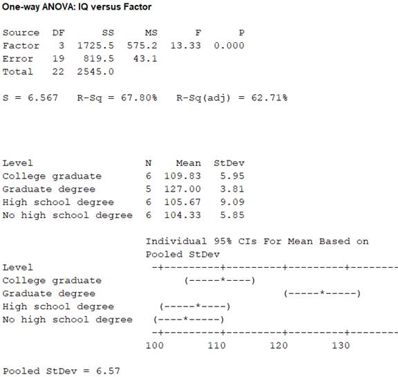
From the MINITAB output, the test valueF is 13.33.
Conclusion:
From the results, the test value is 13.33.
Here, the F-statistic value is greater than the critical value.
That is,
Thus, it can be concluding that, the null hypothesis is rejected.
Hence, there is evidence to reject the claim thatthe mean IQs of the various educational levels of the subjectsare equal. So use Scheffe test for where the difference exists.
Consider,
From the Minitab output, the sample sizes
The means are
The sample variances are
Critical value:
The formula for critical value F1 for the Scheffe test is,
Here, the critical value of F test is 3.13.
Substitute 3.13 for critical value is of F and 3 for k-1 in
Comparison of the means:
The formula for finding
That is,
Comparison between the means
The hypotheses are given below:
Null hypothesis:
Alternative hypothesis:
Rejection region:
The null hypothesis would be rejected if absolute value greater than the critical value.
The formula for comparing the means
Substitute 104.33 and 105.67 for
Thus, the value of
Conclusion:
The value of
Here, the value of
That is,
Thus, the null hypothesis is not rejected.
Hence, there is no significant difference between the means
Comparison between the means
The hypotheses are given below:
Null hypothesis:
Alternative hypothesis:
Rejection region:
The null hypothesis would be rejected if absolute value greater than the critical value.
The formula for comparing the means
Substitute 104.33 and 109.83 for
Thus, the value of
Conclusion:
The value of
Here, the value of
That is,
Thus, the null hypothesis is not rejected.
Hence, there is no significant difference between the means
Comparison between the means
The hypotheses are given below:
Null hypothesis:
Alternative hypothesis:
Rejection region:
The null hypothesis would be rejected if absolute value greater than the critical value.
The formula for comparing the means
Substitute 105.67 and 109.83 for
Thus, the value of
Conclusion:
The value of
Here, the value of
That is,
Thus, the null hypothesis is not rejected.
Hence, there is no significant difference between the means
Comparison between the means
The hypotheses are given below:
Null hypothesis:
Alternative hypothesis:
Rejection region:
The null hypothesis would be rejected if absolute value greater than the critical value.
The formula for comparing the means
Substitute 104.33 and 127.00 for
Thus, the value of
Conclusion:
The value of
Here, the value of
That is,
Thus, the null hypothesis is rejected.
Hence, there is significant difference between the means
Comparison between the means
The hypotheses are given below:
Null hypothesis:
Alternative hypothesis:
Rejection region:
The null hypothesis would be rejected if absolute value greater than the critical value.
The formula for comparing the means
Substitute 105.67 and 127.00 for
Thus, the value of
Conclusion:
The value of
Here, the value of
That is,
Thus, the null hypothesis is rejected.
Hence, there is significant difference between the means
Comparison between the means
The hypotheses are given below:
Null hypothesis:
Alternative hypothesis:
Rejection region:
The null hypothesis would be rejected if absolute value greater than the critical value.
The formula for comparing the means
Substitute 109.83 and 127.00 for
Thus, the value of
Conclusion:
The value of
Here, the value of
That is,
Thus, the null hypothesis is rejected.
Hence, there is significant difference between the means
Justification:
Here, there is significant difference between the means
Want to see more full solutions like this?
Chapter 12 Solutions
ELEMENTARY STATISTICS: STEP BY STEP- ALE


- The following is a list of questions answered correctly on an exam. Calculate the Measures of Central Tendency from the ungrouped data list. NUMBER OF QUESTIONS ANSWERED CORRECTLY ON AN APTITUDE EXAM 112 72 69 97 107 73 92 76 86 73 126 128 118 127 124 82 104 132 134 83 92 108 96 100 92 115 76 91 102 81 95 141 81 80 106 84 119 113 98 75 68 98 115 106 95 100 85 94 106 119arrow_forwardThe following ordered data list shows the data speeds for cell phones used by a telephone company at an airport: A. Calculate the Measures of Central Tendency using the table in point B. B. Are there differences in the measurements obtained in A and C? Why (give at least one justified reason)? 0.8 1.4 1.8 1.9 3.2 3.6 4.5 4.5 4.6 6.2 6.5 7.7 7.9 9.9 10.2 10.3 10.9 11.1 11.1 11.6 11.8 12.0 13.1 13.5 13.7 14.1 14.2 14.7 15.0 15.1 15.5 15.8 16.0 17.5 18.2 20.2 21.1 21.5 22.2 22.4 23.1 24.5 25.7 28.5 34.6 38.5 43.0 55.6 71.3 77.8arrow_forwardIn a company with 80 employees, 60 earn $10.00 per hour and 20 earn $13.00 per hour. a) Determine the average hourly wage. b) In part a), is the same answer obtained if the 60 employees have an average wage of $10.00 per hour? Prove your answer.arrow_forward
- The following ordered data list shows the data speeds for cell phones used by a telephone company at an airport: A. Calculate the Measures of Central Tendency from the ungrouped data list. B. Group the data in an appropriate frequency table. 0.8 1.4 1.8 1.9 3.2 3.6 4.5 4.5 4.6 6.2 6.5 7.7 7.9 9.9 10.2 10.3 10.9 11.1 11.1 11.6 11.8 12.0 13.1 13.5 13.7 14.1 14.2 14.7 15.0 15.1 15.5 15.8 16.0 17.5 18.2 20.2 21.1 21.5 22.2 22.4 23.1 24.5 25.7 28.5 34.6 38.5 43.0 55.6 71.3 77.8arrow_forwardBusinessarrow_forwardhttps://www.hawkeslearning.com/Statistics/dbs2/datasets.htmlarrow_forward
- NC Current Students - North Ce X | NC Canvas Login Links - North ( X Final Exam Comprehensive x Cengage Learning x WASTAT - Final Exam - STAT → C webassign.net/web/Student/Assignment-Responses/submit?dep=36055360&tags=autosave#question3659890_9 Part (b) Draw a scatter plot of the ordered pairs. N Life Expectancy Life Expectancy 80 70 600 50 40 30 20 10 Year of 1950 1970 1990 2010 Birth O Life Expectancy Part (c) 800 70 60 50 40 30 20 10 1950 1970 1990 W ALT 林 $ # 4 R J7 Year of 2010 Birth F6 4+ 80 70 60 50 40 30 20 10 Year of 1950 1970 1990 2010 Birth Life Expectancy Ox 800 70 60 50 40 30 20 10 Year of 1950 1970 1990 2010 Birth hp P.B. KA & 7 80 % 5 H A B F10 711 N M K 744 PRT SC ALT CTRLarrow_forwardHarvard University California Institute of Technology Massachusetts Institute of Technology Stanford University Princeton University University of Cambridge University of Oxford University of California, Berkeley Imperial College London Yale University University of California, Los Angeles University of Chicago Johns Hopkins University Cornell University ETH Zurich University of Michigan University of Toronto Columbia University University of Pennsylvania Carnegie Mellon University University of Hong Kong University College London University of Washington Duke University Northwestern University University of Tokyo Georgia Institute of Technology Pohang University of Science and Technology University of California, Santa Barbara University of British Columbia University of North Carolina at Chapel Hill University of California, San Diego University of Illinois at Urbana-Champaign National University of Singapore McGill…arrow_forwardName Harvard University California Institute of Technology Massachusetts Institute of Technology Stanford University Princeton University University of Cambridge University of Oxford University of California, Berkeley Imperial College London Yale University University of California, Los Angeles University of Chicago Johns Hopkins University Cornell University ETH Zurich University of Michigan University of Toronto Columbia University University of Pennsylvania Carnegie Mellon University University of Hong Kong University College London University of Washington Duke University Northwestern University University of Tokyo Georgia Institute of Technology Pohang University of Science and Technology University of California, Santa Barbara University of British Columbia University of North Carolina at Chapel Hill University of California, San Diego University of Illinois at Urbana-Champaign National University of Singapore…arrow_forward
- A company found that the daily sales revenue of its flagship product follows a normal distribution with a mean of $4500 and a standard deviation of $450. The company defines a "high-sales day" that is, any day with sales exceeding $4800. please provide a step by step on how to get the answers in excel Q: What percentage of days can the company expect to have "high-sales days" or sales greater than $4800? Q: What is the sales revenue threshold for the bottom 10% of days? (please note that 10% refers to the probability/area under bell curve towards the lower tail of bell curve) Provide answers in the yellow cellsarrow_forwardFind the critical value for a left-tailed test using the F distribution with a 0.025, degrees of freedom in the numerator=12, and degrees of freedom in the denominator = 50. A portion of the table of critical values of the F-distribution is provided. Click the icon to view the partial table of critical values of the F-distribution. What is the critical value? (Round to two decimal places as needed.)arrow_forwardA retail store manager claims that the average daily sales of the store are $1,500. You aim to test whether the actual average daily sales differ significantly from this claimed value. You can provide your answer by inserting a text box and the answer must include: Null hypothesis, Alternative hypothesis, Show answer (output table/summary table), and Conclusion based on the P value. Showing the calculation is a must. If calculation is missing,so please provide a step by step on the answers Numerical answers in the yellow cellsarrow_forward
 Glencoe Algebra 1, Student Edition, 9780079039897...AlgebraISBN:9780079039897Author:CarterPublisher:McGraw Hill
 Holt Mcdougal Larson Pre-algebra: Student Edition...AlgebraISBN:9780547587776Author:HOLT MCDOUGALPublisher:HOLT MCDOUGAL
 Big Ideas Math A Bridge To Success Algebra 1: Stu...AlgebraISBN:9781680331141Author:HOUGHTON MIFFLIN HARCOURTPublisher:Houghton Mifflin Harcourt