
Concept explainers
Videos
(a)
To find: The fitted data and the residuals. Also, generate the
(a)
Answer to Problem 22E
Solution: The residuals of the provided data is scattered symmetrically above and below the zero and there is no extreme outlier.
Explanation of Solution
Given: The data provided in the Facebook friends study as,
| Friends | Participant | Score |
| 102 | 1 | 3.8 |
| 102 | 2 | 3.6 |
| 102 | 3 | 3.2 |
| 102 | 4 | 2.4 |
| 102 | 5 | 4.8 |
| 102 | 6 | 3.0 |
| 102 | 7 | 4.2 |
| 102 | 8 | 3.6 |
| 102 | 9 | 3.2 |
| 102 | 10 | 3.0 |
| 102 | 11 | 4.8 |
| 102 | 12 | 3.4 |
| 102 | 13 | 4.8 |
| 102 | 14 | 3.0 |
| 102 | 15 | 4.6 |
| 102 | 16 | 2.8 |
| 102 | 17 | 6.0 |
| 102 | 18 | 2.8 |
| 102 | 19 | 5.2 |
| 102 | 20 | 3.2 |
| 102 | 21 | 4.2 |
| 102 | 22 | 2.2 |
| 102 | 23 | 5.0 |
| 102 | 24 | 4.8 |
| 302 | 25 | 5.0 |
| 302 | 26 | 5.2 |
| 302 | 27 | 5.6 |
| 302 | 28 | 2.6 |
| 302 | 29 | 3.8 |
| 302 | 30 | 4.8 |
| 302 | 31 | 5.6 |
| 302 | 32 | 4.8 |
| 302 | 33 | 6.4 |
| 302 | 34 | 4.8 |
| 302 | 35 | 4.4 |
| 302 | 36 | 6.0 |
| 302 | 37 | 3.8 |
| 302 | 38 | 4.8 |
| 302 | 39 | 4.6 |
| 302 | 40 | 6.0 |
| 302 | 41 | 5.0 |
| 302 | 42 | 3.0 |
| 302 | 43 | 4.4 |
| 302 | 44 | 5.4 |
| 302 | 45 | 5.4 |
| 302 | 46 | 4.6 |
| 302 | 47 | 5.6 |
| 302 | 48 | 5.8 |
| 302 | 49 | 4.2 |
| 302 | 50 | 4.8 |
| 302 | 51 | 5.0 |
| 302 | 52 | 5.2 |
| 302 | 53 | 4.2 |
| 302 | 54 | 5.0 |
| 302 | 55 | 5.8 |
| 302 | 56 | 5.6 |
| 302 | 57 | 3.8 |
| 502 | 58 | 4.6 |
| 502 | 59 | 4.0 |
| 502 | 60 | 4.8 |
| 502 | 61 | 3.0 |
| 502 | 62 | 2.0 |
| 502 | 63 | 5.8 |
| 502 | 64 | 5.6 |
| 502 | 65 | 4.4 |
| 502 | 66 | 4.4 |
| 502 | 67 | 5.6 |
| 502 | 68 | 4.6 |
| 502 | 69 | 5.6 |
| 502 | 70 | 3.0 |
| 502 | 71 | 5.6 |
| 502 | 72 | 3.6 |
| 502 | 73 | 6.8 |
| 502 | 74 | 3.2 |
| 502 | 75 | 4.8 |
| 502 | 76 | 4.6 |
| 502 | 77 | 5.4 |
| 502 | 78 | 4.8 |
| 502 | 79 | 4.8 |
| 502 | 80 | 5.4 |
| 502 | 81 | 3.6 |
| 502 | 82 | 4.8 |
| 502 | 83 | 3.8 |
| 702 | 84 | 3.2 |
| 702 | 85 | 3.6 |
| 702 | 86 | 5.8 |
| 702 | 87 | 1.2 |
| 702 | 88 | 3.8 |
| 702 | 89 | 5.4 |
| 702 | 90 | 3.6 |
| 702 | 91 | 3.4 |
| 702 | 92 | 5.0 |
| 702 | 93 | 5.2 |
| 702 | 94 | 3.6 |
| 702 | 95 | 2.6 |
| 702 | 96 | 7.0 |
| 702 | 97 | 4.4 |
| 702 | 98 | 4.8 |
| 702 | 99 | 5.2 |
| 702 | 100 | 5.4 |
| 702 | 101 | 3.6 |
| 702 | 102 | 1.0 |
| 702 | 103 | 5.0 |
| 702 | 104 | 5.0 |
| 702 | 105 | 6.0 |
| 702 | 106 | 4.2 |
| 702 | 107 | 5.8 |
| 702 | 108 | 3.2 |
| 702 | 109 | 5.4 |
| 702 | 110 | 6.4 |
| 702 | 111 | 4.4 |
| 702 | 112 | 3.0 |
| 702 | 113 | 6.0 |
| 902 | 114 | 4.2 |
| 902 | 115 | 4.6 |
| 902 | 116 | 3.0 |
| 902 | 117 | 2.6 |
| 902 | 118 | 5.2 |
| 902 | 119 | 5.2 |
| 902 | 120 | 1.6 |
| 902 | 121 | 5.0 |
| 902 | 122 | 4.4 |
| 902 | 123 | 5.0 |
| 902 | 124 | 3.6 |
| 902 | 125 | 4.2 |
| 902 | 126 | 5.0 |
| 902 | 127 | 3.4 |
| 902 | 128 | 3.6 |
| 902 | 129 | 5.0 |
| 902 | 130 | 3.2 |
| 902 | 131 | 2.4 |
| 902 | 132 | 4.8 |
| 902 | 133 | 3.6 |
| 902 | 134 | 4.2 |
Calculation:
Use Minitab to find the residuals, of the provided data as below:
Step1: Enter the provided data in the worksheet.
Step2: Select stat >ANOVA>one-way analysis of variance.
Step3: Select Score in the Response and Friends in the Factor.
Step4: Click on Graphs and select the Residual verses fitand then press OK.
Step5: Select Store residual and Store fit.
Step6: Press OK.
Theobtained output of fitted data and the residual stored in the data file as below:
| Friends | Participant | Score | RESI1 | FITS1 |
| 102 | 1 | 3.8 | -0.01667 | 3.816667 |
| 102 | 2 | 3.6 | -0.21667 | 3.816667 |
| 102 | 3 | 3.2 | -0.61667 | 3.816667 |
| 102 | 4 | 2.4 | -1.41667 | 3.816667 |
| 102 | 5 | 4.8 | 0.983333 | 3.816667 |
| 102 | 6 | 3.0 | -0.81667 | 3.816667 |
| 102 | 7 | 4.2 | 0.383333 | 3.816667 |
| 102 | 8 | 3.6 | -0.21667 | 3.816667 |
| 102 | 9 | 3.2 | -0.61667 | 3.816667 |
| 102 | 10 | 3.0 | -0.81667 | 3.816667 |
| 102 | 11 | 4.8 | 0.983333 | 3.816667 |
| 102 | 12 | 3.4 | -0.41667 | 3.816667 |
| 102 | 13 | 4.8 | 0.983333 | 3.816667 |
| 102 | 14 | 3.0 | -0.81667 | 3.816667 |
| 102 | 15 | 4.6 | 0.783333 | 3.816667 |
| 102 | 16 | 2.8 | -1.01667 | 3.816667 |
| 102 | 17 | 6.0 | 2.183333 | 3.816667 |
| 102 | 18 | 2.8 | -1.01667 | 3.816667 |
| 102 | 19 | 5.2 | 1.383333 | 3.816667 |
| 102 | 20 | 3.2 | -0.61667 | 3.816667 |
| 102 | 21 | 4.2 | 0.383333 | 3.816667 |
| 102 | 22 | 2.2 | -1.61667 | 3.816667 |
| 102 | 23 | 5.0 | 1.183333 | 3.816667 |
| 102 | 24 | 4.8 | 0.983333 | 3.816667 |
| 302 | 25 | 5.0 | 0.121212 | 4.878788 |
| 302 | 26 | 5.2 | 0.321212 | 4.878788 |
| 302 | 27 | 5.6 | 0.721212 | 4.878788 |
| 302 | 28 | 2.6 | -2.27879 | 4.878788 |
| 302 | 29 | 3.8 | -1.07879 | 4.878788 |
| 302 | 30 | 4.8 | -0.07879 | 4.878788 |
| 302 | 31 | 5.6 | 0.721212 | 4.878788 |
| 302 | 32 | 4.8 | -0.07879 | 4.878788 |
| 302 | 33 | 6.4 | 1.521212 | 4.878788 |
| 302 | 34 | 4.8 | -0.07879 | 4.878788 |
| 302 | 35 | 4.4 | -0.47879 | 4.878788 |
| 302 | 36 | 6.0 | 1.121212 | 4.878788 |
| 302 | 37 | 3.8 | -1.07879 | 4.878788 |
| 302 | 38 | 4.8 | -0.07879 | 4.878788 |
| 302 | 39 | 4.6 | -0.27879 | 4.878788 |
| 302 | 40 | 6.0 | 1.121212 | 4.878788 |
| 302 | 41 | 5.0 | 0.121212 | 4.878788 |
| 302 | 42 | 3.0 | -1.87879 | 4.878788 |
| 302 | 43 | 4.4 | -0.47879 | 4.878788 |
| 302 | 44 | 5.4 | 0.521212 | 4.878788 |
| 302 | 45 | 5.4 | 0.521212 | 4.878788 |
| 302 | 46 | 4.6 | -0.27879 | 4.878788 |
| 302 | 47 | 5.6 | 0.721212 | 4.878788 |
| 302 | 48 | 5.8 | 0.921212 | 4.878788 |
| 302 | 49 | 4.2 | -0.67879 | 4.878788 |
| 302 | 50 | 4.8 | -0.07879 | 4.878788 |
| 302 | 51 | 5.0 | 0.121212 | 4.878788 |
| 302 | 52 | 5.2 | 0.321212 | 4.878788 |
| 302 | 53 | 4.2 | -0.67879 | 4.878788 |
| 302 | 54 | 5.0 | 0.121212 | 4.878788 |
| 302 | 55 | 5.8 | 0.921212 | 4.878788 |
| 302 | 56 | 5.6 | 0.721212 | 4.878788 |
| 302 | 57 | 3.8 | -1.07879 | 4.878788 |
| 502 | 58 | 4.6 | 0.038462 | 4.561538 |
| 502 | 59 | 4.0 | -0.56154 | 4.561538 |
| 502 | 60 | 4.8 | 0.238462 | 4.561538 |
| 502 | 61 | 3.0 | -1.56154 | 4.561538 |
| 502 | 62 | 2.0 | -2.56154 | 4.561538 |
| 502 | 63 | 5.8 | 1.238462 | 4.561538 |
| 502 | 64 | 5.6 | 1.038462 | 4.561538 |
| 502 | 65 | 4.4 | -0.16154 | 4.561538 |
| 502 | 66 | 4.4 | -0.16154 | 4.561538 |
| 502 | 67 | 5.6 | 1.038462 | 4.561538 |
| 502 | 68 | 4.6 | 0.038462 | 4.561538 |
| 502 | 69 | 5.6 | 1.038462 | 4.561538 |
| 502 | 70 | 3.0 | -1.56154 | 4.561538 |
| 502 | 71 | 5.6 | 1.038462 | 4.561538 |
| 502 | 72 | 3.6 | -0.96154 | 4.561538 |
| 502 | 73 | 6.8 | 2.238462 | 4.561538 |
| 502 | 74 | 3.2 | -1.36154 | 4.561538 |
| 502 | 75 | 4.8 | 0.238462 | 4.561538 |
| 502 | 76 | 4.6 | 0.038462 | 4.561538 |
| 502 | 77 | 5.4 | 0.838462 | 4.561538 |
| 502 | 78 | 4.8 | 0.238462 | 4.561538 |
| 502 | 79 | 4.8 | 0.238462 | 4.561538 |
| 502 | 80 | 5.4 | 0.838462 | 4.561538 |
| 502 | 81 | 3.6 | -0.96154 | 4.561538 |
| 502 | 82 | 4.8 | 0.238462 | 4.561538 |
| 502 | 83 | 3.8 | -0.76154 | 4.561538 |
| 702 | 84 | 3.2 | -1.20667 | 4.406667 |
| 702 | 85 | 3.6 | -0.80667 | 4.406667 |
| 702 | 86 | 5.8 | 1.393333 | 4.406667 |
| 702 | 87 | 1.2 | -3.20667 | 4.406667 |
| 702 | 88 | 3.8 | -0.60667 | 4.406667 |
| 702 | 89 | 5.4 | 0.993333 | 4.406667 |
| 702 | 90 | 3.6 | -0.80667 | 4.406667 |
| 702 | 91 | 3.4 | -1.00667 | 4.406667 |
| 702 | 92 | 5.0 | 0.593333 | 4.406667 |
| 702 | 93 | 5.2 | 0.793333 | 4.406667 |
| 702 | 94 | 3.6 | -0.80667 | 4.406667 |
| 702 | 95 | 2.6 | -1.80667 | 4.406667 |
| 702 | 96 | 7.0 | 2.593333 | 4.406667 |
| 702 | 97 | 4.4 | -0.00667 | 4.406667 |
| 702 | 98 | 4.8 | 0.393333 | 4.406667 |
| 702 | 99 | 5.2 | 0.793333 | 4.406667 |
| 702 | 100 | 5.4 | 0.993333 | 4.406667 |
| 702 | 101 | 3.6 | -0.80667 | 4.406667 |
| 702 | 102 | 1.0 | -3.40667 | 4.406667 |
| 702 | 103 | 5.0 | 0.593333 | 4.406667 |
| 702 | 104 | 5.0 | 0.593333 | 4.406667 |
| 702 | 105 | 6.0 | 1.593333 | 4.406667 |
| 702 | 106 | 4.2 | -0.20667 | 4.406667 |
| 702 | 107 | 5.8 | 1.393333 | 4.406667 |
| 702 | 108 | 3.2 | -1.20667 | 4.406667 |
| 702 | 109 | 5.4 | 0.993333 | 4.406667 |
| 702 | 110 | 6.4 | 1.993333 | 4.406667 |
| 702 | 111 | 4.4 | -0.00667 | 4.406667 |
| 702 | 112 | 3.0 | -1.40667 | 4.406667 |
| 702 | 113 | 6.0 | 1.593333 | 4.406667 |
| 902 | 114 | 4.2 | 0.209524 | 3.990476 |
| 902 | 115 | 4.6 | 0.609524 | 3.990476 |
| 902 | 116 | 3.0 | -0.99048 | 3.990476 |
| 902 | 117 | 2.6 | -1.39048 | 3.990476 |
| 902 | 118 | 5.2 | 1.209524 | 3.990476 |
| 902 | 119 | 5.2 | 1.209524 | 3.990476 |
| 902 | 120 | 1.6 | -2.39048 | 3.990476 |
| 902 | 121 | 5.0 | 1.009524 | 3.990476 |
| 902 | 122 | 4.4 | 0.409524 | 3.990476 |
| 902 | 123 | 5.0 | 1.009524 | 3.990476 |
| 902 | 124 | 3.6 | -0.39048 | 3.990476 |
| 902 | 125 | 4.2 | 0.209524 | 3.990476 |
| 902 | 126 | 5.0 | 1.009524 | 3.990476 |
| 902 | 127 | 3.4 | -0.59048 | 3.990476 |
| 902 | 128 | 3.6 | -0.39048 | 3.990476 |
| 902 | 129 | 5.0 | 1.009524 | 3.990476 |
| 902 | 130 | 3.2 | -0.79048 | 3.990476 |
| 902 | 131 | 2.4 | -1.59048 | 3.990476 |
| 902 | 132 | 4.8 | 0.809524 | 3.990476 |
| 902 | 133 | 3.6 | -0.39048 | 3.990476 |
| 902 | 134 | 4.2 | 0.209524 | 3.990476 |
The scatterplot of the residuals versus the group variable is,
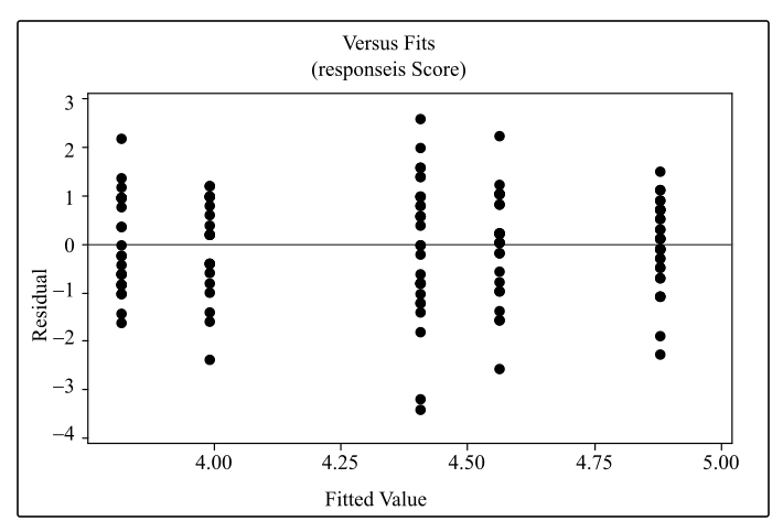
Interpretation: From the above graph, it is observed that the scatter plot of the residuals is symmetrically scattered below and above the zero and there are two outliers below the zero but these are not the extreme outliers.
(b)
Whether the spread of the residual of each group is relatively equal or not.
(b)
Answer to Problem 22E
Solution: Yes, the spread of the residual of each group is relatively equal.
Explanation of Solution
From the scatterplot of the residuals versus the group variables in part (a), it is observed that the residuals are symmetrically scattered below and above the zero. It implies that the spread of the residual of each group is relatively equal.
(c)
To graph: The Normal quantile plot of the residuals obtained in part (a) and identify whether it is normal or not.
(c)
Explanation of Solution
Graph:
Use Minitab to graph the Normal quantile plot as below:
Step1: Enter the provided data in the worksheet.
Step2: Select stat> ANOVA>one-way analysis of variance.
Step3: Select Score in the Response and Friends in the Factor.
Step4: Click on Graphs and select the Normal plot of residuals and then press OK.
Step5: Press OK.
The obtained graph is,
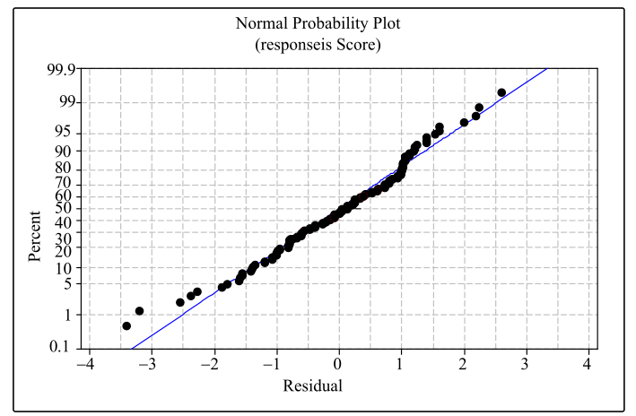
Interpretation: From the obtained graph, it is observed that the normal quantile plot is nearly fitted to the line. Hence, the residual is approximately normal.
Want to see more full solutions like this?
Chapter 12 Solutions
EBK INTRODUCTION TO THE PRACTICE OF STA


- I need help with this problem and an explanation of the solution for the image described below. (Statistics: Engineering Probabilities)arrow_forwardI need help with this problem and an explanation of the solution for the image described below. (Statistics: Engineering Probabilities)arrow_forwardI need help with this problem and an explanation of the solution for the image described below. (Statistics: Engineering Probabilities)arrow_forward
- I need help with this problem and an explanation of the solution for the image described below. (Statistics: Engineering Probabilities)arrow_forwardI need help with this problem and an explanation of the solution for the image described below. (Statistics: Engineering Probabilities)arrow_forward3. Consider the following regression model: Yi Bo+B1x1 + = ···· + ßpxip + Єi, i = 1, . . ., n, where are i.i.d. ~ N (0,0²). (i) Give the MLE of ẞ and σ², where ẞ = (Bo, B₁,..., Bp)T. (ii) Derive explicitly the expressions of AIC and BIC for the above linear regression model, based on their general formulae.arrow_forward
- How does the width of prediction intervals for ARMA(p,q) models change as the forecast horizon increases? Grows to infinity at a square root rate Depends on the model parameters Converges to a fixed value Grows to infinity at a linear ratearrow_forwardConsider the AR(3) model X₁ = 0.6Xt-1 − 0.4Xt-2 +0.1Xt-3. What is the value of the PACF at lag 2? 0.6 Not enough information None of these values 0.1 -0.4 이arrow_forwardSuppose you are gambling on a roulette wheel. Each time the wheel is spun, the result is one of the outcomes 0, 1, and so on through 36. Of these outcomes, 18 are red, 18 are black, and 1 is green. On each spin you bet $5 that a red outcome will occur and $1 that the green outcome will occur. If red occurs, you win a net $4. (You win $10 from red and nothing from green.) If green occurs, you win a net $24. (You win $30 from green and nothing from red.) If black occurs, you lose everything you bet for a loss of $6. a. Use simulation to generate 1,000 plays from this strategy. Each play should indicate the net amount won or lost. Then, based on these outcomes, calculate a 95% confidence interval for the total net amount won or lost from 1,000 plays of the game. (Round your answers to two decimal places and if your answer is negative value, enter "minus" sign.) I worked out the Upper Limit, but I can't seem to arrive at the correct answer for the Lower Limit. What is the Lower Limit?…arrow_forward
- Let us suppose we have some article reported on a study of potential sources of injury to equine veterinarians conducted at a university veterinary hospital. Forces on the hand were measured for several common activities that veterinarians engage in when examining or treating horses. We will consider the forces on the hands for two tasks, lifting and using ultrasound. Assume that both sample sizes are 6, the sample mean force for lifting was 6.2 pounds with standard deviation 1.5 pounds, and the sample mean force for using ultrasound was 6.4 pounds with standard deviation 0.3 pounds. Assume that the standard deviations are known. Suppose that you wanted to detect a true difference in mean force of 0.25 pounds on the hands for these two activities. Under the null hypothesis, 40 0. What level of type II error would you recommend here? = Round your answer to four decimal places (e.g. 98.7654). Use α = 0.05. β = 0.0594 What sample size would be required? Assume the sample sizes are to be…arrow_forwardConsider the hypothesis test Ho: 0 s² = = 4.5; s² = 2.3. Use a = 0.01. = σ against H₁: 6 > σ2. Suppose that the sample sizes are n₁ = 20 and 2 = 8, and that (a) Test the hypothesis. Round your answers to two decimal places (e.g. 98.76). The test statistic is fo = 1.96 The critical value is f = 6.18 Conclusion: fail to reject the null hypothesis at a = 0.01. (b) Construct the confidence interval on 02/2/622 which can be used to test the hypothesis: (Round your answer to two decimal places (e.g. 98.76).) 035arrow_forwardUsing the method of sections need help solving this please explain im stuckarrow_forward
 Big Ideas Math A Bridge To Success Algebra 1: Stu...AlgebraISBN:9781680331141Author:HOUGHTON MIFFLIN HARCOURTPublisher:Houghton Mifflin Harcourt
 Glencoe Algebra 1, Student Edition, 9780079039897...AlgebraISBN:9780079039897Author:CarterPublisher:McGraw Hill
 Functions and Change: A Modeling Approach to Coll...AlgebraISBN:9781337111348Author:Bruce Crauder, Benny Evans, Alan NoellPublisher:Cengage Learning
 Holt Mcdougal Larson Pre-algebra: Student Edition...AlgebraISBN:9780547587776Author:HOLT MCDOUGALPublisher:HOLT MCDOUGAL
 College AlgebraAlgebraISBN:9781305115545Author:James Stewart, Lothar Redlin, Saleem WatsonPublisher:Cengage Learning