
Concept explainers
Videos
a.
Find
a.
Answer to Problem 10E
The intercept
The slope
Explanation of Solution
Calculation:
The given information is that the sample data consists of 8 values for x and y.
Slope or
where,
r represents the
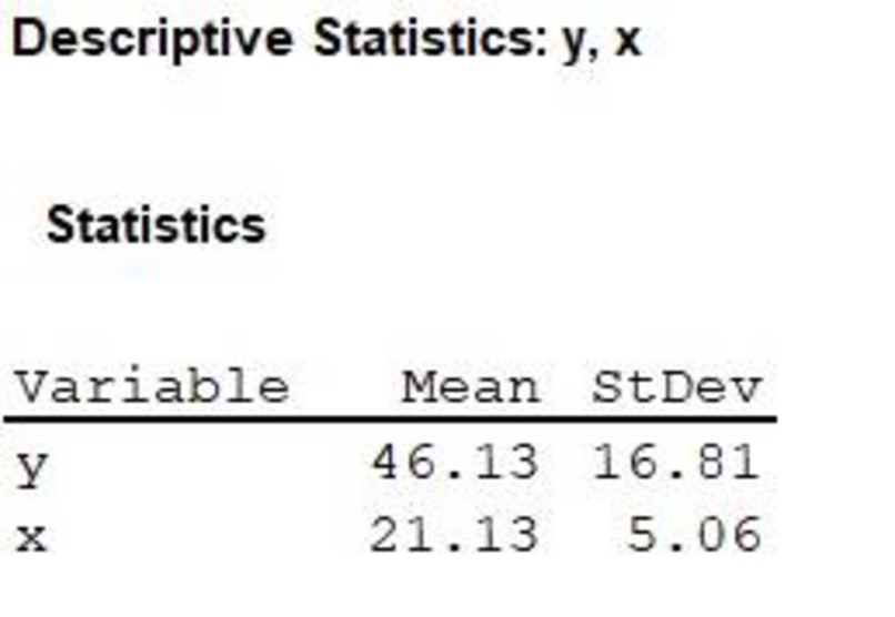
Software procedure:
Step-by-step procedure to find the
- Choose Stat > Basic Statistics > Display
Descriptive Statistics . - In Variables enter the columns of y and x.
- Choose Options Statistics, select Mean and Standard deviation.
- Click OK.
Output obtained from MINITAB is given below:
Correlation:
Where,
n represents the sample size.
The table shows the calculation of correlation:
| x | y | |||||
| 23 | 51 | 1.87 | 4.87 | 0.369565 | 0.289709 | 0.107066 |
| 16 | 22 | –5.13 | –24.13 | –1.01383 | –1.43546 | 1.455313 |
| 17 | 56 | –4.13 | 9.87 | –0.81621 | 0.587151 | –0.47924 |
| 19 | 34 | –2.13 | –12.13 | –0.42095 | –0.72159 | 0.303754 |
| 30 | 67 | 8.87 | 20.87 | 1.752964 | 1.241523 | 2.176345 |
| 19 | 59 | –2.13 | 12.87 | –0.42095 | 0.765616 | –0.32228 |
| 18 | 55 | –3.13 | 8.87 | –0.61858 | 0.527662 | –0.3264 |
| 27 | 25 | 5.87 | –21.13 | 1.160079 | –1.25699 | –1.45821 |
| Total | 1.456 |
Thus, the correlation is
Substitute r as 0.208,
Thus, the slope
Intercept or
Substitute
Thus, the intercept
b.
Find the predicted value
b.
Answer to Problem 10E
The predicted value
Explanation of Solution
Calculation:
The given value of x is 25.
The estimated regression equation is
Substitute x as 25,
Thus, the predicted value
c.
Find the residual standard deviation
c.
Answer to Problem 10E
The residual standard deviation
Explanation of Solution
Calculation:
The residual standard deviation
Where,
n represents the
Use the estimated regression equation to find the predicted value of y for each value of x.
| y |  | ||
| 51 | 47.423 | 3.577 | 12.79493 |
| 22 | 42.586 | –20.586 | 423.7834 |
| 56 | 43.277 | 12.723 | 161.8747 |
| 34 | 44.659 | –10.659 | 113.6143 |
| 67 | 52.26 | 14.74 | 217.2676 |
| 59 | 44.659 | 14.341 | 205.6643 |
| 55 | 43.968 | 11.032 | 121.705 |
| 25 | 50.187 | –25.187 | 634.385 |
| Total | 1,891.09 |
Substitute
Thus, the residual standard deviation
d.
Find the sum of squares for x.
d.
Answer to Problem 10E
The sum of squares for x is 178.8752.
Explanation of Solution
Calculation:
The table shows the calculation of sum of squares for x:
| x | ||
| 23 | 1.87 | 3.4969 |
| 16 | -5.13 | 26.3169 |
| 17 | -4.13 | 17.0569 |
| 19 | -2.13 | 4.5369 |
| 30 | 8.87 | 78.6769 |
| 19 | -2.13 | 4.5369 |
| 18 | -3.13 | 9.7969 |
| 27 | 5.87 | 34.4569 |
| Total | 178.8752 |
Thus, the sum of squares for x is 178.8752.
e.
Find the critical value for a 95% confidence or prediction interval.
e.
Answer to Problem 10E
The critical value for a 95% confidence or prediction interval is 2.447.
Explanation of Solution
Calculation:
Critical value:
Software procedure:
Step-by-step procedure to find the critical value using MINITAB is given below:
- Choose Graph > Probability Distribution Plot choose View Probability > OK.
- From Distribution, choose ‘t’ distribution.
- In Degrees of freedom, enter 4.
- Click the Shaded Area tab.
- Choose Probability and Two tail for the region of the curve to shade.
- Enter the Probability value as 0.05.
- Click OK.
Output obtained from MINITAB is given below:
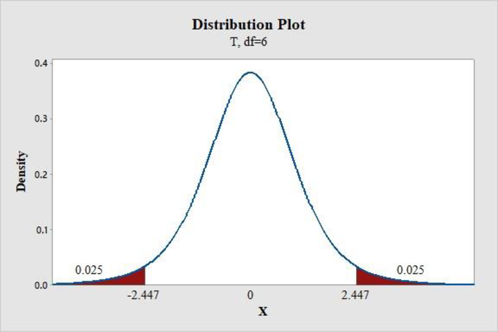
Thus, the critical value for a 95% confidence or prediction interval is 2.447.
f.
Construct the 95% confidence interval for the mean response for the given value of x.
f.
Answer to Problem 10E
The 95% confidence interval for the mean response for the given value of x is
Explanation of Solution
Calculation:
The given value of x is 25.
Software procedure:
Step-by-step procedure to construct the 95% confidence interval for the mean response for the given value of x is given below:
- Choose Stat > Regression > Regression.
- In Response, enter the column containing the y.
- In Predictors, enter the columns containing the x.
- Click OK.
- Choose Stat > Regression > Regression>Predict.
- Choose Enter the individual values.
- Enter the x as 25.
- Click OK.
Output obtained from MINITAB is given below:
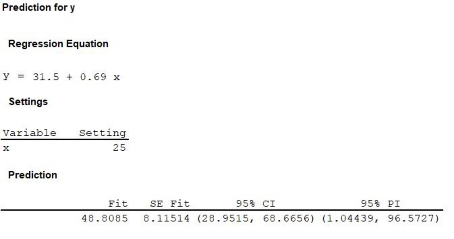
Interpretation:
Thus, the 95% confidence interval for the mean response for the given value of x is
g.
Construct the 95% prediction interval for the individual response for the given value of x.
g.
Answer to Problem 10E
The 95% prediction interval for the individual response for the given value of x is
Explanation of Solution
From the MINITAB output obtained in the previous part (f) it can be observed that the 95% prediction interval for the individual response for the given value of x is
Want to see more full solutions like this?
Chapter 11 Solutions
Essential Statistics


- A psychology researcher conducted a Chi-Square Test of Independence to examine whether there is a relationship between college students’ year in school (Freshman, Sophomore, Junior, Senior) and their preferred coping strategy for academic stress (Problem-Focused, Emotion-Focused, Avoidance). The test yielded the following result: image.png Interpret the results of this analysis. In your response, clearly explain: Whether the result is statistically significant and why. What this means about the relationship between year in school and coping strategy. What the researcher should conclude based on these findings.arrow_forwardA school counselor is conducting a research study to examine whether there is a relationship between the number of times teenagers report vaping per week and their academic performance, measured by GPA. The counselor collects data from a sample of high school students. Write the null and alternative hypotheses for this study. Clearly state your hypotheses in terms of the correlation between vaping frequency and academic performance. EditViewInsertFormatToolsTable 12pt Paragrapharrow_forwardA smallish urn contains 25 small plastic bunnies – 7 of which are pink and 18 of which are white. 10 bunnies are drawn from the urn at random with replacement, and X is the number of pink bunnies that are drawn. (a) P(X = 5) ≈ (b) P(X<6) ≈ The Whoville small urn contains 100 marbles – 60 blue and 40 orange. The Grinch sneaks in one night and grabs a simple random sample (without replacement) of 15 marbles. (a) The probability that the Grinch gets exactly 6 blue marbles is [ Select ] ["≈ 0.054", "≈ 0.043", "≈ 0.061"] . (b) The probability that the Grinch gets at least 7 blue marbles is [ Select ] ["≈ 0.922", "≈ 0.905", "≈ 0.893"] . (c) The probability that the Grinch gets between 8 and 12 blue marbles (inclusive) is [ Select ] ["≈ 0.801", "≈ 0.760", "≈ 0.786"] . The Whoville small urn contains 100 marbles – 60 blue and 40 orange. The Grinch sneaks in one night and grabs a simple random sample (without replacement) of 15 marbles. (a)…arrow_forward
- Suppose an experiment was conducted to compare the mileage(km) per litre obtained by competing brands of petrol I,II,III. Three new Mazda, three new Toyota and three new Nissan cars were available for experimentation. During the experiment the cars would operate under same conditions in order to eliminate the effect of external variables on the distance travelled per litre on the assigned brand of petrol. The data is given as below: Brands of Petrol Mazda Toyota Nissan I 10.6 12.0 11.0 II 9.0 15.0 12.0 III 12.0 17.4 13.0 (a) Test at the 5% level of significance whether there are signi cant differences among the brands of fuels and also among the cars. [10] (b) Compute the standard error for comparing any two fuel brands means. Hence compare, at the 5% level of significance, each of fuel brands II, and III with the standard fuel brand I. [10] �arrow_forwardBusiness discussarrow_forwardWhat would you say about a set of quantitative bivariate data whose linear correlation is -1? What would a scatter diagram of the data look like? (5 points)arrow_forward
- Business discussarrow_forwardAnalyze the residuals of a linear regression model and select the best response. yes, the residual plot does not show a curve no, the residual plot shows a curve yes, the residual plot shows a curve no, the residual plot does not show a curve I answered, "No, the residual plot shows a curve." (and this was incorrect). I am not sure why I keep getting these wrong when the answer seems obvious. Please help me understand what the yes and no references in the answer.arrow_forwarda. Find the value of A.b. Find pX(x) and py(y).c. Find pX|y(x|y) and py|X(y|x)d. Are x and y independent? Why or why not?arrow_forward
- Analyze the residuals of a linear regression model and select the best response.Criteria is simple evaluation of possible indications of an exponential model vs. linear model) no, the residual plot does not show a curve yes, the residual plot does not show a curve yes, the residual plot shows a curve no, the residual plot shows a curve I selected: yes, the residual plot shows a curve and it is INCORRECT. Can u help me understand why?arrow_forwardYou have been hired as an intern to run analyses on the data and report the results back to Sarah; the five questions that Sarah needs you to address are given below. please do it step by step on excel Does there appear to be a positive or negative relationship between price and screen size? Use a scatter plot to examine the relationship. Determine and interpret the correlation coefficient between the two variables. In your interpretation, discuss the direction of the relationship (positive, negative, or zero relationship). Also discuss the strength of the relationship. Estimate the relationship between screen size and price using a simple linear regression model and interpret the estimated coefficients. (In your interpretation, tell the dollar amount by which price will change for each unit of increase in screen size). Include the manufacturer dummy variable (Samsung=1, 0 otherwise) and estimate the relationship between screen size, price and manufacturer dummy as a multiple…arrow_forwardHere is data with as the response variable. x y54.4 19.124.9 99.334.5 9.476.6 0.359.4 4.554.4 0.139.2 56.354 15.773.8 9-156.1 319.2Make a scatter plot of this data. Which point is an outlier? Enter as an ordered pair, e.g., (x,y). (x,y)= Find the regression equation for the data set without the outlier. Enter the equation of the form mx+b rounded to three decimal places. y_wo= Find the regression equation for the data set with the outlier. Enter the equation of the form mx+b rounded to three decimal places. y_w=arrow_forward
 Glencoe Algebra 1, Student Edition, 9780079039897...AlgebraISBN:9780079039897Author:CarterPublisher:McGraw Hill
 Holt Mcdougal Larson Pre-algebra: Student Edition...AlgebraISBN:9780547587776Author:HOLT MCDOUGALPublisher:HOLT MCDOUGAL
 Big Ideas Math A Bridge To Success Algebra 1: Stu...AlgebraISBN:9781680331141Author:HOUGHTON MIFFLIN HARCOURTPublisher:Houghton Mifflin Harcourt