
Concept explainers
Videos
a.
Calculate the values of
a.
Answer to Problem 43E
The value of
The value of
The value of
The value of
Explanation of Solution
Calculation:
The number of years of service (x) and the hourly wages ($) (y) of the five employees of a small company are given.
Denote
Software procedure:
Step-by-step procedure to obtain the descriptive statistics using the MINITAB software:
- Choose Stat > Basic Statistics > Display Descriptive Statistics, click OK.
- In Variables, enter the columns of x and y.
- Choose Statistics, select Mean, Standard deviation and click OK.
- Click OK.
Output using the MINITAB software is given below:
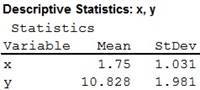
From the above output, it is evident that the value of
b.
Find the
b.
Answer to Problem 43E
The
Explanation of Solution
Calculation:
Correlation:
The correlation coefficient, r, between ordered pairs of variables, (x, y) having sample means
Software procedure:
Step-by-step procedure to obtain the correlation using the MINITAB software:
- Choose Stat > Basic Statistics > Correlation.
- In Variables, enter the columns of x and y.
- Click OK.
Output using the MINITAB software is given below:
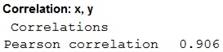
From the output, the correlation coefficient between the years of service and the hourly wages is 0.906.
c.
Find the sample mean and the sample standard deviation of the hourly wages, if each employee is given a raise of $1.00 per hour.
c.
Answer to Problem 43E
The sample mean of the hourly wages, if each employee is given a raise of $1.00 per hour is 11.828.
The sample standard deviation of the hourly wages, if each employee is given a raise of $1.00 per hour is 1.981.
Explanation of Solution
Calculation:
Denote
The calculation for
| y | |
| 9.50 | 10.50 |
| 8.23 | 9.23 |
| 10.95 | 11.95 |
| 12.70 | 13.70 |
| 12.75 | 13.75 |
Descriptive statistics:
Software procedure:
Step-by-step procedure to obtain the descriptive statistics using the MINITAB software:
- Choose Stat > Basic Statistics > Display Descriptive Statistics, click OK.
- In Variables, enter the columns of y1.
- Choose Statistics, select Mean, Standard deviation and click OK.
- Click OK.
Output using the MINITAB software is given below:
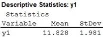
From the above output, it is evident that the sample mean of the hourly wages, if each employee is given a raise of $1.00 per hour is 11.828 and the sample standard deviation of the hourly wages, if each employee is given a raise of $1.00 per hour is 1.981.
d.
Identify the effects of increasing each value of y by 1 on the values of
d.
Answer to Problem 43E
The average hourly wage
The standard deviation
Explanation of Solution
Interpretation:
From part a, the value of average hourly wages,
From part c, the value of sample mean of the hourly wages, if each employee is given a raise of $1.00 per hour is 11.828.
Now,
Hence, it is evident that the average hourly wage has increased by $1.00 due to increasing each value of y by 1.
From part a, the value of standard deviation of hourly wages,
From part c, the value of sample standard deviation , if each employee is given a raise of $1.00 per hour is 1.981.
Evidently, the standard deviation has remained unchanged due to increasing each value of y by 1.
e.
Find the correlation coefficient between the years of service and the increased hourly wages.
Explain the reason the correlation coefficient remains unchanged even when the values of y change.
e.
Answer to Problem 43E
The correlation coefficient between the years of service and the increased hourly wages is 0.906.
Explanation of Solution
Calculation:
Correlation:
Software procedure:
Step-by-step procedure to obtain the correlation using the MINITAB software:
- Choose Stat > Basic Statistics > Correlation.
- In Variables, enter the columns of x and y1.
- Click OK.
Output using the MINITAB software is given below:
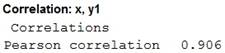
From the output, the correlation coefficient between the years of service and the increased hourly wages is 0.906.
Consider the formula for the correlation coefficient, r:
Now, each y increases and becomes
Again, as observed from part d, the mean of the increased hourly wages is
Replace these in the formula for the correlation coefficient:
It is observed that the correlation coefficient is independent of the change of origin.
Hence, the correlation coefficient remains unchanged even when the values of y change.
f.
Find the sample mean and the sample standard deviation of the service period, if it is expressed in terms of months.
f.
Answer to Problem 43E
The sample mean of the hourly wages, of the service period, if it is expressed in terms of months is 21.
The sample standard deviation of the hourly wages, of the service period, if it is expressed in terms of months is 12.37.
Explanation of Solution
Calculation:
Denote
The calculation for
| x | |
| 0.5 | 6 |
| 1.0 | 12 |
| 1.75 | 21 |
| 2.5 | 30 |
| 3.0 | 36 |
Descriptive statistics:
Software procedure:
Step-by-step procedure to obtain the descriptive statistics using the MINITAB software:
- Choose Stat > Basic Statistics > Display Descriptive Statistics, click OK.
- In Variables, enter the columns of x1.
- Choose Statistics, select Mean, Standard deviation and click OK.
- Click OK.
Output using the MINITAB software is given below:
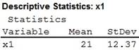
From the above output, it is evident that the sample mean of the hourly wages, of the service period, if it is expressed in terms of months is 21 and the sample standard deviation of the hourly wages, of the service period, if it is expressed in terms of months is 12.37.
g.
Identify the effects of multiplying each value of x by 12 on the values of
g.
Answer to Problem 43E
The average service period in months has been multiplied by 12 due to multiplying each value of x by 12.
The standard deviation has been multiplied by 12 due to multiplying each value of x by 12.
Explanation of Solution
Interpretation:
From part a, the average service period in years,
From part f, the average service period in months is 21.
Now,
Hence, it is evident that the average hourly wage has increased by $1.00 due to increasing each value of y by 1.
From part a, the value of standard deviation of service period in years,
From part c, the value of sample standard deviation of service period in months is 12.37.
Now,
In other words,
Evidently, the standard deviation has been multiplied by 12 due to multiplying each value of x by 12.
h.
Find the correlation coefficient between the months of service and the hourly wages.
Explain the reason the correlation coefficient remains unchanged even when the values of
h.
Answer to Problem 43E
The correlation coefficient between the months of service and the increased hourly wages is 0.906.
Explanation of Solution
Calculation:
Correlation:
Software procedure:
Step-by-step procedure to obtain the correlation using the MINITAB software:
- Choose Stat > Basic Statistics > Correlation.
- In Variables, enter the columns of x1 and y.
- Click OK.
Output using the MINITAB software is given below:
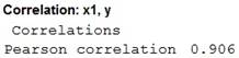
From the output, the correlation coefficient between the months of service and the increased hourly wages is 0.906.
Consider the formula for the correlation coefficient, r:
Now, each x is multiplied by 12 and becomes
Again, as observed from part d, the mean of the months of service is
Replace these in the formula for the correlation coefficient:
It is observed that the correlation coefficient is independent of the changes of origin and scale.
Hence, the correlation coefficient remains unchanged even when the values of
i.
Find the effect of adding a constant to each x-value or to each y-value on the correlation coefficient.
i.
Answer to Problem 43E
If a constant is added to each x-value or to each y-value, the correlation coefficient is unchanged.
Explanation of Solution
Interpretation:
The correlation coefficient is independent of the change of origin of the variables. Adding a constant to each x-value or to each y-value implies a change in origin of x or y.
Hence, if a constant is added to each x-value or to each y-value, the correlation coefficient is unchanged.
Correlation:
The correlation coefficient, r, between ordered pairs of variables, (x, y) having sample means
j.
Find the effect of multiplying a positive constant to each x-value or to each y-value on the correlation coefficient.
j.
Answer to Problem 43E
If each x-value or each y-value is multiplied by a positive constant, the correlation coefficient is unchanged.
Explanation of Solution
Interpretation:
The correlation coefficient is independent of the change of scale of the variables. Multiplying a positive constant with each x-value or each y-value changes the scale of x or y.
Hence, if each x-value or each y-value is multiplied by a positive constant, the correlation coefficient is unchanged.
Want to see more full solutions like this?
Chapter 11 Solutions
Essential Statistics


- For each of the time series, construct a line chart of the data and identify the characteristics of the time series (that is, random, stationary, trend, seasonal, or cyclical). Year Month Rate (%)2009 Mar 8.72009 Apr 9.02009 May 9.42009 Jun 9.52009 Jul 9.52009 Aug 9.62009 Sep 9.82009 Oct 10.02009 Nov 9.92009 Dec 9.92010 Jan 9.82010 Feb 9.82010 Mar 9.92010 Apr 9.92010 May 9.62010 Jun 9.42010 Jul 9.52010 Aug 9.52010 Sep 9.52010 Oct 9.52010 Nov 9.82010 Dec 9.32011 Jan 9.12011 Feb 9.02011 Mar 8.92011 Apr 9.02011 May 9.02011 Jun 9.12011 Jul 9.02011 Aug 9.02011 Sep 9.02011 Oct 8.92011 Nov 8.62011 Dec 8.52012 Jan 8.32012 Feb 8.32012 Mar 8.22012 Apr 8.12012 May 8.22012 Jun 8.22012 Jul 8.22012 Aug 8.12012 Sep 7.82012 Oct…arrow_forwardFor each of the time series, construct a line chart of the data and identify the characteristics of the time series (that is, random, stationary, trend, seasonal, or cyclical). Date IBM9/7/2010 $125.959/8/2010 $126.089/9/2010 $126.369/10/2010 $127.999/13/2010 $129.619/14/2010 $128.859/15/2010 $129.439/16/2010 $129.679/17/2010 $130.199/20/2010 $131.79 a. Construct a line chart of the closing stock prices data. Choose the correct chart below.arrow_forwardFor each of the time series, construct a line chart of the data and identify the characteristics of the time series (that is, random, stationary, trend, seasonal, or cyclical) Date IBM9/7/2010 $125.959/8/2010 $126.089/9/2010 $126.369/10/2010 $127.999/13/2010 $129.619/14/2010 $128.859/15/2010 $129.439/16/2010 $129.679/17/2010 $130.199/20/2010 $131.79arrow_forward
- 1. A consumer group claims that the mean annual consumption of cheddar cheese by a person in the United States is at most 10.3 pounds. A random sample of 100 people in the United States has a mean annual cheddar cheese consumption of 9.9 pounds. Assume the population standard deviation is 2.1 pounds. At a = 0.05, can you reject the claim? (Adapted from U.S. Department of Agriculture) State the hypotheses: Calculate the test statistic: Calculate the P-value: Conclusion (reject or fail to reject Ho): 2. The CEO of a manufacturing facility claims that the mean workday of the company's assembly line employees is less than 8.5 hours. A random sample of 25 of the company's assembly line employees has a mean workday of 8.2 hours. Assume the population standard deviation is 0.5 hour and the population is normally distributed. At a = 0.01, test the CEO's claim. State the hypotheses: Calculate the test statistic: Calculate the P-value: Conclusion (reject or fail to reject Ho): Statisticsarrow_forward21. find the mean. and variance of the following: Ⓒ x(t) = Ut +V, and V indepriv. s.t U.VN NL0, 63). X(t) = t² + Ut +V, U and V incepires have N (0,8) Ut ①xt = e UNN (0162) ~ X+ = UCOSTE, UNNL0, 62) SU, Oct ⑤Xt= 7 where U. Vindp.rus +> ½ have NL, 62). ⑥Xn = ΣY, 41, 42, 43, ... Yn vandom sample K=1 Text with mean zen and variance 6arrow_forwardA psychology researcher conducted a Chi-Square Test of Independence to examine whether there is a relationship between college students’ year in school (Freshman, Sophomore, Junior, Senior) and their preferred coping strategy for academic stress (Problem-Focused, Emotion-Focused, Avoidance). The test yielded the following result: image.png Interpret the results of this analysis. In your response, clearly explain: Whether the result is statistically significant and why. What this means about the relationship between year in school and coping strategy. What the researcher should conclude based on these findings.arrow_forward
- A school counselor is conducting a research study to examine whether there is a relationship between the number of times teenagers report vaping per week and their academic performance, measured by GPA. The counselor collects data from a sample of high school students. Write the null and alternative hypotheses for this study. Clearly state your hypotheses in terms of the correlation between vaping frequency and academic performance. EditViewInsertFormatToolsTable 12pt Paragrapharrow_forwardA smallish urn contains 25 small plastic bunnies – 7 of which are pink and 18 of which are white. 10 bunnies are drawn from the urn at random with replacement, and X is the number of pink bunnies that are drawn. (a) P(X = 5) ≈ (b) P(X<6) ≈ The Whoville small urn contains 100 marbles – 60 blue and 40 orange. The Grinch sneaks in one night and grabs a simple random sample (without replacement) of 15 marbles. (a) The probability that the Grinch gets exactly 6 blue marbles is [ Select ] ["≈ 0.054", "≈ 0.043", "≈ 0.061"] . (b) The probability that the Grinch gets at least 7 blue marbles is [ Select ] ["≈ 0.922", "≈ 0.905", "≈ 0.893"] . (c) The probability that the Grinch gets between 8 and 12 blue marbles (inclusive) is [ Select ] ["≈ 0.801", "≈ 0.760", "≈ 0.786"] . The Whoville small urn contains 100 marbles – 60 blue and 40 orange. The Grinch sneaks in one night and grabs a simple random sample (without replacement) of 15 marbles. (a)…arrow_forwardSuppose an experiment was conducted to compare the mileage(km) per litre obtained by competing brands of petrol I,II,III. Three new Mazda, three new Toyota and three new Nissan cars were available for experimentation. During the experiment the cars would operate under same conditions in order to eliminate the effect of external variables on the distance travelled per litre on the assigned brand of petrol. The data is given as below: Brands of Petrol Mazda Toyota Nissan I 10.6 12.0 11.0 II 9.0 15.0 12.0 III 12.0 17.4 13.0 (a) Test at the 5% level of significance whether there are signi cant differences among the brands of fuels and also among the cars. [10] (b) Compute the standard error for comparing any two fuel brands means. Hence compare, at the 5% level of significance, each of fuel brands II, and III with the standard fuel brand I. [10] �arrow_forward
 MATLAB: An Introduction with ApplicationsStatisticsISBN:9781119256830Author:Amos GilatPublisher:John Wiley & Sons Inc
 Probability and Statistics for Engineering and th...StatisticsISBN:9781305251809Author:Jay L. DevorePublisher:Cengage Learning
 Statistics for The Behavioral Sciences (MindTap C...StatisticsISBN:9781305504912Author:Frederick J Gravetter, Larry B. WallnauPublisher:Cengage Learning
 Elementary Statistics: Picturing the World (7th E...StatisticsISBN:9780134683416Author:Ron Larson, Betsy FarberPublisher:PEARSON
 The Basic Practice of StatisticsStatisticsISBN:9781319042578Author:David S. Moore, William I. Notz, Michael A. FlignerPublisher:W. H. Freeman
 Introduction to the Practice of StatisticsStatisticsISBN:9781319013387Author:David S. Moore, George P. McCabe, Bruce A. CraigPublisher:W. H. Freeman