Mathematical Statistics with Applications
7th Edition
ISBN: 9780495110811
Author: Dennis Wackerly, William Mendenhall, Richard L. Scheaffer
Publisher: Cengage Learning
expand_more
expand_more
format_list_bulleted
Concept explainers
Textbook Question
Chapter 11.3, Problem 14E
J. H. Matis and T. E. Wehrly report the following table of data on the proportion of green sunfish that survive a fixed level of thermal pollution for varying lengths of time.
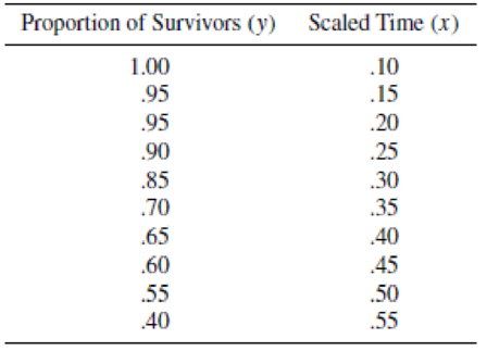
- a Fit the linear model Y = β0 + β1x + ε. Give your interpretation.
- b Plot the points and graph the result of part (a). Does the line fit through the points?
Expert Solution & Answer
Want to see the full answer?
Check out a sample textbook solution
Students have asked these similar questions
1. For the data in table 3.1,
a. Fit a linear model using the score 0,2,4,6.
b. Interpret the numerical values of the slope and intercept.
c. Refit the linear model using scores 0,1,2,3
Chapter 11 Solutions
Mathematical Statistics with Applications
Ch. 11.3 - If 0 and 1 are the least-squares estimates for the...Ch. 11.3 - Prob. 2ECh. 11.3 - Fit a straight line to the five data points in the...Ch. 11.3 - Auditors are often required to compare the audited...Ch. 11.3 - Prob. 5ECh. 11.3 - Applet Exercise Refer to Exercises 11.2 and 11.5....Ch. 11.3 - Prob. 7ECh. 11.3 - Laboratory experiments designed to measure LC50...Ch. 11.3 - Prob. 9ECh. 11.3 - Suppose that we have postulated the model...
Ch. 11.3 - Some data obtained by C.E. Marcellari on the...Ch. 11.3 - Processors usually preserve cucumbers by...Ch. 11.3 - J. H. Matis and T. E. Wehrly report the following...Ch. 11.4 - a Derive the following identity:...Ch. 11.4 - An experiment was conducted to observe the effect...Ch. 11.4 - Prob. 17ECh. 11.4 - Prob. 18ECh. 11.4 - A study was conducted to determine the effects of...Ch. 11.4 - Suppose that Y1, Y2,,Yn are independent normal...Ch. 11.4 - Under the assumptions of Exercise 11.20, find...Ch. 11.4 - Prob. 22ECh. 11.5 - Use the properties of the least-squares estimators...Ch. 11.5 - Do the data in Exercise 11.19 present sufficient...Ch. 11.5 - Use the properties of the least-squares estimators...Ch. 11.5 - Let Y1, Y2, . . . , Yn be as given in Exercise...Ch. 11.5 - Prob. 30ECh. 11.5 - Using a chemical procedure called differential...Ch. 11.5 - Prob. 32ECh. 11.5 - Prob. 33ECh. 11.5 - Prob. 34ECh. 11.6 - For the simple linear regression model Y = 0 + 1x...Ch. 11.6 - Prob. 36ECh. 11.6 - Using the model fit to the data of Exercise 11.8,...Ch. 11.6 - Refer to Exercise 11.3. Find a 90% confidence...Ch. 11.6 - Refer to Exercise 11.16. Find a 95% confidence...Ch. 11.6 - Refer to Exercise 11.14. Find a 90% confidence...Ch. 11.6 - Prob. 41ECh. 11.7 - Suppose that the model Y=0+1+ is fit to the n data...Ch. 11.7 - Prob. 43ECh. 11.7 - Prob. 44ECh. 11.7 - Prob. 45ECh. 11.7 - Refer to Exercise 11.16. Find a 95% prediction...Ch. 11.7 - Refer to Exercise 11.14. Find a 95% prediction...Ch. 11.8 - The accompanying table gives the peak power load...Ch. 11.8 - Prob. 49ECh. 11.8 - Prob. 50ECh. 11.8 - Prob. 51ECh. 11.8 - Prob. 52ECh. 11.8 - Prob. 54ECh. 11.8 - Prob. 55ECh. 11.8 - Prob. 57ECh. 11.8 - Prob. 58ECh. 11.8 - Prob. 59ECh. 11.8 - Prob. 60ECh. 11.9 - Refer to Example 11.10. Find a 90% prediction...Ch. 11.9 - Prob. 62ECh. 11.9 - Prob. 63ECh. 11.9 - Prob. 64ECh. 11.9 - Prob. 65ECh. 11.10 - Refer to Exercise 11.3. Fit the model suggested...Ch. 11.10 - Prob. 67ECh. 11.10 - Fit the quadratic model Y=0+1x+2x2+ to the data...Ch. 11.10 - The manufacturer of Lexus automobiles has steadily...Ch. 11.10 - a Calculate SSE and S2 for Exercise 11.4. Use the...Ch. 11.12 - Consider the general linear model...Ch. 11.12 - Prob. 72ECh. 11.12 - Prob. 73ECh. 11.12 - An experiment was conducted to investigate the...Ch. 11.12 - Prob. 75ECh. 11.12 - The results that follow were obtained from an...Ch. 11.13 - Prob. 77ECh. 11.13 - Prob. 78ECh. 11.13 - Prob. 79ECh. 11.14 - Prob. 80ECh. 11.14 - Prob. 81ECh. 11.14 - Prob. 82ECh. 11.14 - Prob. 83ECh. 11.14 - Prob. 84ECh. 11.14 - Prob. 85ECh. 11.14 - Prob. 86ECh. 11.14 - Prob. 87ECh. 11.14 - Prob. 88ECh. 11.14 - Refer to the three models given in Exercise 11.88....Ch. 11.14 - Prob. 90ECh. 11.14 - Prob. 91ECh. 11.14 - Prob. 92ECh. 11.14 - Prob. 93ECh. 11.14 - Prob. 94ECh. 11 - At temperatures approaching absolute zero (273C),...Ch. 11 - A study was conducted to determine whether a...Ch. 11 - Prob. 97SECh. 11 - Prob. 98SECh. 11 - Prob. 99SECh. 11 - Prob. 100SECh. 11 - Prob. 102SECh. 11 - Prob. 103SECh. 11 - An experiment was conducted to determine the...Ch. 11 - Prob. 105SECh. 11 - Prob. 106SECh. 11 - Prob. 107SE
Knowledge Booster
Learn more about
Need a deep-dive on the concept behind this application? Look no further. Learn more about this topic, statistics and related others by exploring similar questions and additional content below.Similar questions
- Find the slope of the line containing each pair of points in Exercise 2. a 2,-3 and 2,5 c -4,1 and 4,5 b 3,-2 and -7,-2 d x-2,y-3 and x+4,y+5arrow_forwardCholesterol. The age, x, and LDL cholesterol level, y, of two men are given by the points (18,69) and (27,122) . Find a linear equation that models the relationship between age and LDL cholesterol level.arrow_forwardWhat is interpolation when using a linear model?arrow_forward
- Demand for Candy Bars In this problem you will determine a linear demand equation that describes the demand for candy bars in your class. Survey your classmates to determine what price they would be willing to pay for a candy bar. Your survey form might look like the sample to the left. a Make a table of the number of respondents who answered yes at each price level. b Make a scatter plot of your data. c Find and graph the regression line y=mp+b, which gives the number of respondents y who would buy a candy bar if the price were p cents. This is the demand equation. Why is the slope m negative? d What is the p-intercept of the demand equation? What does this intercept tell you about pricing candy bars? Would you buy a candy bar from the vending machine in the hallway if the price is as indicated. Price Yes or No 50 75 1.00 1.25 1.50 1.75 2.00arrow_forwardSports The ordered pairs below give the winning times (in seconds) of the women’s 100-meter freestyle in the Olympics from 1984 through 2012. 1984,55.92 2000,53.83 1988,54.93 2004,53.84 1992,54.64 2008,53.12 1996,54.50 2012,53.00 (a) Sketch a scatter plot of the data. Let y represent the winning time (in seconds) and let t=84 represent 1984. (b) Sketch the line that you think best approximates the data and find an equation of the line. (c) Use the regression feature of a graphing utility to find the equation of the least squares regression line that fits the data. (d) Compare the linear model you found in part (b) with the linear model you found in part (c).arrow_forward
arrow_back_ios
arrow_forward_ios
Recommended textbooks for you
 Glencoe Algebra 1, Student Edition, 9780079039897...AlgebraISBN:9780079039897Author:CarterPublisher:McGraw Hill
 Elementary AlgebraAlgebraISBN:9780998625713Author:Lynn Marecek, MaryAnne Anthony-SmithPublisher:OpenStax - Rice University
 College AlgebraAlgebraISBN:9781305115545Author:James Stewart, Lothar Redlin, Saleem WatsonPublisher:Cengage Learning
 Trigonometry (MindTap Course List)TrigonometryISBN:9781305652224Author:Charles P. McKeague, Mark D. TurnerPublisher:Cengage Learning
 Intermediate AlgebraAlgebraISBN:9781285195728Author:Jerome E. Kaufmann, Karen L. SchwittersPublisher:Cengage Learning

Glencoe Algebra 1, Student Edition, 9780079039897...
Algebra
ISBN:9780079039897
Author:Carter
Publisher:McGraw Hill


Elementary Algebra
Algebra
ISBN:9780998625713
Author:Lynn Marecek, MaryAnne Anthony-Smith
Publisher:OpenStax - Rice University

College Algebra
Algebra
ISBN:9781305115545
Author:James Stewart, Lothar Redlin, Saleem Watson
Publisher:Cengage Learning

Trigonometry (MindTap Course List)
Trigonometry
ISBN:9781305652224
Author:Charles P. McKeague, Mark D. Turner
Publisher:Cengage Learning

Intermediate Algebra
Algebra
ISBN:9781285195728
Author:Jerome E. Kaufmann, Karen L. Schwitters
Publisher:Cengage Learning
Correlation Vs Regression: Difference Between them with definition & Comparison Chart; Author: Key Differences;https://www.youtube.com/watch?v=Ou2QGSJVd0U;License: Standard YouTube License, CC-BY
Correlation and Regression: Concepts with Illustrative examples; Author: LEARN & APPLY : Lean and Six Sigma;https://www.youtube.com/watch?v=xTpHD5WLuoA;License: Standard YouTube License, CC-BY