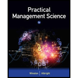
Practical Management Science
5th Edition
ISBN: 9781305250901
Author: Wayne L. Winston, S. Christian Albright
Publisher: Cengage Learning
expand_more
expand_more
format_list_bulleted
Concept explainers
Textbook Question
Chapter 11.2, Problem 5P
In Example 11.2, the gamma distribution was used to model the skewness to the right of the lifetime distribution. Experiment to see whether the triangular distribution could have been used instead. Let its minimum value be 0, and choose its most likely and maximum values so that this triangular distribution has approximately the same mean and standard deviation as the gamma distribution in the example. (Use @RISK’s Define Distributions window and trial and error to do this.) Then run the simulation and comment on similarities or differences between your outputs and the outputs in the example.
Expert Solution & Answer
Want to see the full answer?
Check out a sample textbook solution
Students have asked these similar questions
Can you guys help me with this? Thank you!
Here's the question: Compared to the CONSTRAINT model, how has the network changed? How do you plan to add contingency to your network? Please answer this thoroughly
Here's the what-if scenario: Assume that the LA warehouse becomes temporarily or even indefinitely disabled since facing a large-scale labor disruption. Re-optimize the network considering this new constraint.
Here's the scenario comparison analysis:
Scenario Constraint Scenario vs What-if Scenario
Summary The Constraint Scenario exhibits a higher total cost of $7,424,575.45 compared to the What-if Scenario's total cost of $6,611,905.60, signifying a difference of approximately $812,669.85, which indicates a more expensive operation in the Constraint Scenario. The average service time is slightly higher in the Constraint Scenario (0.72 days vs. 0.70 days), suggesting that the What-if Scenario provides a marginally quicker service. Moreover, the average end-to-end service time…
Can you guys help me with this? Thank you!
Here's the question: Compared to the CONSTRAINT model, how has the network changed? How do you plan to add contingency to your network? Please answer this throughly
Here's the what-if scenario: Assume that Dallas plant has lost power. It cannot serve the DCs anymore and has to remain locked indefinitely. Re-optimize the network considering this new constraint.
Here's the scenario comparison analysis:
Scenario Constraint Scenario vs What-if Scenario
Summary In comparing the Constraint Scenario to the What-if Scenario, a few key differences highlight the efficiencies evident in the supply chain. Firstly, the total cost in the Constraint Scenario is lower at $7,424,575.45, while the What-if Scenario incurs a total cost of $7,486,369.12, resulting in a cost delta of $61,793.67. Additionally, although both scenarios exhibit the same average service time of 0.72 days, the What-if Scenario has a more favorable average end-to-end service time of 2.41…
Employee In-Service Training
ASSIGNMENT: In-Service Training. The intern is required to plan and implement two in-service training sessions for
employees. Each in-service should last at least 10 but not more than 30 minutes and should be given to all employees affected.
The preceptor or supervisor/unit manager must approve all in-service topics.
1) One presentation should be related to a policy or procedure of any kind (e.g. proper use of equipment);
2) The second presentation must be related to sanitation or safety.
For each in-service presentation, the intern must develop a written class plan and a visual aid (may be a handout, poster,
PowerPoint slide presentation, etc.) appropriate to the life experiences, cultural diversity and educational background of the
target audience. The intern must also measure behavior change. Note, this cannot be measured by a written pre- and post-
test. That would be measuring knowledge. The intern mustactually observe and document that the learners…
Chapter 11 Solutions
Practical Management Science
Ch. 11.2 - If the number of competitors in Example 11.1...Ch. 11.2 - In Example 11.1, the possible profits vary from...Ch. 11.2 - Referring to Example 11.1, if the average bid for...Ch. 11.2 - See how sensitive the results in Example 11.2 are...Ch. 11.2 - In Example 11.2, the gamma distribution was used...Ch. 11.2 - Prob. 6PCh. 11.2 - In Example 11.3, suppose you want to run five...Ch. 11.2 - In Example 11.3, if a batch fails to pass...Ch. 11.3 - Rerun the new car simulation from Example 11.4,...Ch. 11.3 - Rerun the new car simulation from Example 11.4,...
Ch. 11.3 - In the cash balance model from Example 11.5, the...Ch. 11.3 - Prob. 12PCh. 11.3 - Prob. 13PCh. 11.3 - The simulation output from Example 11.6 indicates...Ch. 11.3 - Prob. 15PCh. 11.3 - Referring to the retirement example in Example...Ch. 11.3 - A European put option allows an investor to sell a...Ch. 11.3 - Prob. 18PCh. 11.3 - Prob. 19PCh. 11.3 - Based on Kelly (1956). You currently have 100....Ch. 11.3 - Amanda has 30 years to save for her retirement. At...Ch. 11.3 - In the financial world, there are many types of...Ch. 11.3 - Suppose you currently have a portfolio of three...Ch. 11.3 - If you own a stock, buying a put option on the...Ch. 11.3 - Prob. 25PCh. 11.3 - Prob. 26PCh. 11.3 - Prob. 27PCh. 11.3 - Prob. 28PCh. 11.4 - Prob. 29PCh. 11.4 - Seas Beginning sells clothing by mail order. An...Ch. 11.4 - Based on Babich (1992). Suppose that each week...Ch. 11.4 - The customer loyalty model in Example 11.9 assumes...Ch. 11.4 - Prob. 33PCh. 11.4 - Suppose that GLC earns a 2000 profit each time a...Ch. 11.4 - Prob. 35PCh. 11.5 - A martingale betting strategy works as follows....Ch. 11.5 - The game of Chuck-a-Luck is played as follows: You...Ch. 11.5 - You have 5 and your opponent has 10. You flip a...Ch. 11.5 - Assume a very good NBA team has a 70% chance of...Ch. 11.5 - Consider the following card game. The player and...Ch. 11.5 - Prob. 42PCh. 11 - Prob. 44PCh. 11 - You now have 10,000, all of which is invested in a...Ch. 11 - Prob. 46PCh. 11 - Prob. 47PCh. 11 - Based on Marcus (1990). The Balboa mutual fund has...Ch. 11 - Prob. 50PCh. 11 - Prob. 52PCh. 11 - The annual demand for Prizdol, a prescription drug...Ch. 11 - Prob. 54PCh. 11 - The DC Cisco office is trying to predict the...Ch. 11 - Prob. 56PCh. 11 - Prob. 58PCh. 11 - You are considering a 10-year investment project....Ch. 11 - Prob. 61PCh. 11 - An automobile manufacturer is considering whether...Ch. 11 - Prob. 63PCh. 11 - Prob. 65PCh. 11 - Rework the previous problem for a case in which...Ch. 11 - Prob. 68PCh. 11 - The Tinkan Company produces one-pound cans for the...Ch. 11 - Prob. 70PCh. 11 - In this version of dice blackjack, you toss a...Ch. 11 - Prob. 76PCh. 11 - It is January 1 of year 0, and Merck is trying to...Ch. 11 - Suppose you are an HR (human resources) manager at...Ch. 11 - You are an avid basketball fan, and you would like...Ch. 11 - Suppose you are a financial analyst and your...Ch. 11 - Software development is an inherently risky and...Ch. 11 - Health care is continually in the news. Can (or...
Knowledge Booster
Learn more about
Need a deep-dive on the concept behind this application? Look no further. Learn more about this topic, operations-management and related others by exploring similar questions and additional content below.Similar questions
- A small furniture manufacturer produces tables and chairs. Each product must go through three stages of the manufacturing process – assembly, finishing, and inspection. Each table requires 3 hours of assembly, 2 hours of finishing, and 1 hour of inspection. The profit per table is $120 while the profit per chair is $80. Currently, each week there are 200 hours of assembly time available, 180 hours of finishing time, and 40 hours of inspection time. Linear programming is to be used to develop a production schedule. Define the variables as follows: T = number of tables produced each week C= number of chairs produced each week According to the above information, what would the objective function be? (a) Maximize T+C (b) Maximize 120T + 80C (c) Maximize 200T+200C (d) Minimize 6T+5C (e) none of the above According to the information provided in Question 17, which of the following would be a necessary constraint in the problem? (a) T+C ≤ 40 (b) T+C ≤ 200 (c) T+C ≤ 180 (d) 120T+80C ≥ 1000…arrow_forwardAs much detail as possible. Dietary Management- Nursing Home Don't add any fill-in-the-blanksarrow_forwardMenu Planning Instructions Use the following questions and points as a guide to completing this assignment. The report should be typed. Give a copy to the facility preceptor. Submit a copy in your Foodservice System Management weekly submission. 1. Are there any federal regulations and state statutes or rules with which they must comply? Ask preceptor about regulations that could prescribe a certain amount of food that must be kept on hand for emergencies, etc. Is the facility accredited by any agency such as Joint Commission? 2. Describe the kind of menu the facility uses (may include standard select menu, menu specific to station, non-select, select, room service, etc.) 3. What type of foodservice does the facility have? This could be various stations to choose from, self-serve, 4. conventional, cook-chill, assembly-serve, etc. Are there things about the facility or system that place a constraint on the menu to be served? Consider how patients/guests are served (e.g. do they serve…arrow_forward
- Work with the chef and/or production manager to identify a menu item (or potential menu item) for which a standardized recipe is needed. Record the recipe with which you started and expand it to meet the number of servings required by the facility. Develop an evaluation rubric. Conduct an evaluation of the product. There should be three or more people evaluating the product for quality. Write a brief report of this activity • Product chosen and the reason why it was selected When and where the facility could use the product The standardized recipe sheet or card 。 o Use the facility's format or Design one of your own using a form of your choice; be sure to include the required elements • • Recipe title Yield and portion size Cooking time and temperature Ingredients and quantities Specify AP or EP Procedures (direction)arrow_forwardASSIGNMENT: Inventory, Answer the following questions 1. How does the facility survey inventory? 2. Is there a perpetual system in place? 3. How often do they do a physical inventory? 4. Participate in taking inventory. 5. Which type of stock system does the facility use? A. Minimum stock- includes a safety factor for replenishing stock B. Maximum stock- equal to a safety stock plus estimated usage (past usage and forecasts) C. Mini-max-stock allowed to deplete to a safety level before a new order is submitted to bring up inventory up to max again D. Par stock-stock brought up to the par level each time an order is placed regardless of the amount on hand at the time of order E. Other-(describe) Choose an appropriate product and determine how much of an item should be ordered. Remember the formula is: Demand during lead time + safety stock = amount to order Cost out an inventory according to data supplied. Remember that to do this, you will need to take an inventory, and will need to…arrow_forwardHuman Relations, Systems, and Organization Assignments ORGANIZATION: Review the organization chart for the facility • Draw an organization chart for the department. • . Identify and explain the relationships of different units in the organization and their importance to maintain the food service department's mission. Include a copy in your weekly submission. There is a feature in PowerPoint for doing this should you want to use it. JOB ORGANIZATION: ⚫ A job description is a broad, general, and written statement for a specific job, based on the findings of a job analysis. It generally includes duties, purpose, responsibilities, scope, and working conditions of a job along with the job's title, and the name or designation of the person to whom the employee reports. Job description usually forms the basis of job specification. • Work with your preceptor or supervisor to identify a position for which you will write a job description. Include a copy of the job description you write in your…arrow_forward
arrow_back_ios
SEE MORE QUESTIONS
arrow_forward_ios
Recommended textbooks for you
 Practical Management ScienceOperations ManagementISBN:9781337406659Author:WINSTON, Wayne L.Publisher:Cengage,

Practical Management Science
Operations Management
ISBN:9781337406659
Author:WINSTON, Wayne L.
Publisher:Cengage,
Single Exponential Smoothing & Weighted Moving Average Time Series Forecasting; Author: Matt Macarty;https://www.youtube.com/watch?v=IjETktmL4Kg;License: Standard YouTube License, CC-BY
Introduction to Forecasting - with Examples; Author: Dr. Bharatendra Rai;https://www.youtube.com/watch?v=98K7AG32qv8;License: Standard Youtube License