Videos
a.
Check whether the data provide convincing support for the claim that, on average, male teenager drivers exceed the speed limit by more than do female teenage drivers.
a.
Answer to Problem 18E
The conclusion is that the data provide convincing support for the claim that, on average, male teenager drivers exceed the speed limit by more than do female teenage drivers.
Explanation of Solution
Calculation:
The data are based on the speed limit for male and female drivers.
Step 1:
In this context,
Step 2:
Null hypothesis:
Step 3:
Alternative hypothesis:
Step 4:
Significance level,
It is given that the significance level,
Step 5:
Test statistic:
Step 6:
The assumption for the two-sample t-test:
- The random samples should be collected independently.
- The sample sizes should be large. That is, each sample size is at least 30 or the populations are approximately normally distributed.
It is assumed that the distribution of the speed limit for male and female drivers is normally distributed.
Boxplot:
Software procedure:
Step-by-step procedure to obtain a boxplot using MINITAB software:
- Choose Graphs > Boxplot.
- Under Multiple Y’s, choose Simple.
- In Graph variables, enter the column of Male Driver and Female Driver.
- In Scale, choose Transpose values and categorical scales.
- Click OK in all dialogue boxes.
Output using MINITAB software is given below:
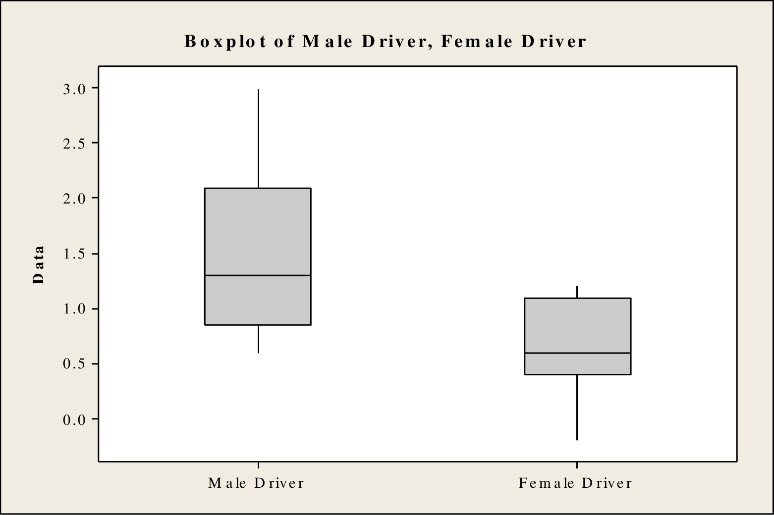
Any lack of symmetric that appears in the boxplot is acceptable for the given sample size because the sample size is larger.
From the boxplot, it is clear that the distribution of the speed limit for male drivers is skewed right and the distribution of the speed limit for female drivers is skewed left. Based on the sample size, the normality condition is satisfied. Morevoer, random samples are collected independently. Therefore, the assumptions are satisfied. It is reasonable to use the data for a two-sample t test.
Step 7:
Test statistic:
Software procedure:
Step-by-step procedure to obtain the P-value and test statistic using MINITAB software:
- Choose Stat > Basic Statistics > 2 sample t.
- Choose Samples in different columns.
- In sample 1, enter the column of Male Driver.
- In sample 2, enter the column of Female Driver.
- Choose Options.
- In Confidence level, enter 95.
- In Alternative, select greater than.
- Click OK in all the dialogue boxes.
Output obtained using MINITAB software is given below:
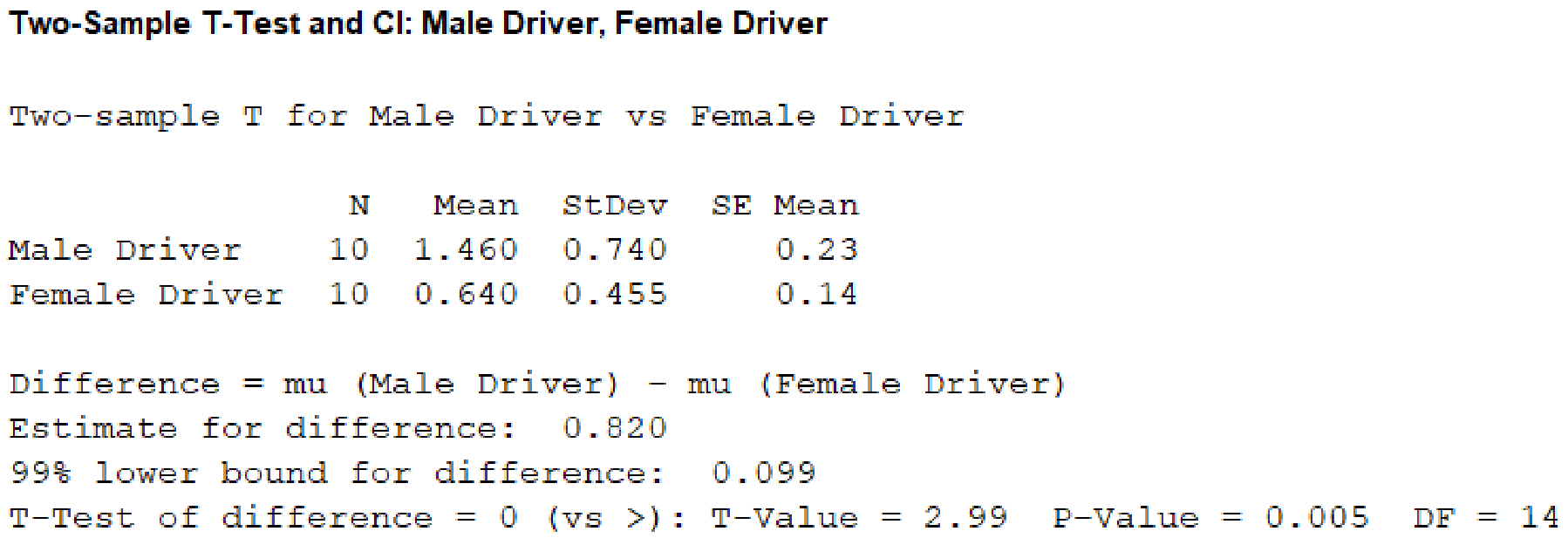
From the given MINITAB output, the value of the test statistic is 2.99.
Step 8:
P-value:
From the MINITAB output, the P-value is 0.005.
Step 9:
Decision rule:
If the
Here, the
That is,
The decision is that the null hypothesis is rejected.
Conclusion:
Hence, the data provide convincing support for the claim that, on average, male teenager drivers exceed the speed limit by more than do female teenage drivers.
b.
(i)
Check whether there is sufficient evidence to conclude that the average number of miles per hour over the speed limit is greater for male drivers with male passengers than it is for male drivers with female passengers.
(ii)
Check whether there is sufficient evidence to conclude that the average number of miles per hour over the speed limit is greater for female drivers with male passengers than it is for female drivers with female passengers.
(iii)
Check whether there is sufficient evidence to conclude that the average number of miles per hour over the speed limit is smaller for male drivers with female passengers than it is for female drivers with male passengers.
b.
Answer to Problem 18E
(i)
The conclusion is that there is sufficient evidence to conclude that the average number of miles per hour over the speed limit is greater for male drivers with male passengers than it is for male drivers with female passengers.
(ii)
The conclusion is that there is sufficient evidence to conclude that the average number of miles per hour over the speed limit is greater for female drivers with male passengers than it is for female drivers with female passengers.
(iii)
The conclusion is that there is sufficient evidence to conclude that the average number of miles per hour over the speed limit is smaller for male drivers with female passengers than it is for female drivers with male passengers.
Explanation of Solution
Calculation:
(i)
Step 1:
In this context,
Step 2:
Null hypothesis:
Step 3:
Alternative hypothesis:
Step 4:
Significance level,
It is given that the significance level
Step 5:
Test statistic:
Step 6:
Assumptions for the two-sample t-test:
- The random samples should be collected independently.
- The sample sizes should be large. That is, each sample size must be at least 30.
Assumption in this particular problem:
- Data are collected independently.
- The sample sizes are large.
Here, both sample sizes are greater than 30.
Therefore, the assumptions are satisfied.
Step 7:
Test statistic:
Software procedure:
Step-by-step procedure to obtain the P-value and test statistic using MINITAB software:
- Choose Stat > Basic Statistics > 2 sample t.
- Choose Summarized data.
- In sample 1, enter Sample size as 40, Mean as 5.2, Standard deviation as 0.8.
- In sample 2, enter Sample size as 40, Mean as 0.3, Standard deviation as 0.8.
- Choose Options.
- In Confidence level, enter 99.
- In Alternative, select greater than.
- Click OK in all the dialogue boxes.
Output obtained using MINITAB software is given below:
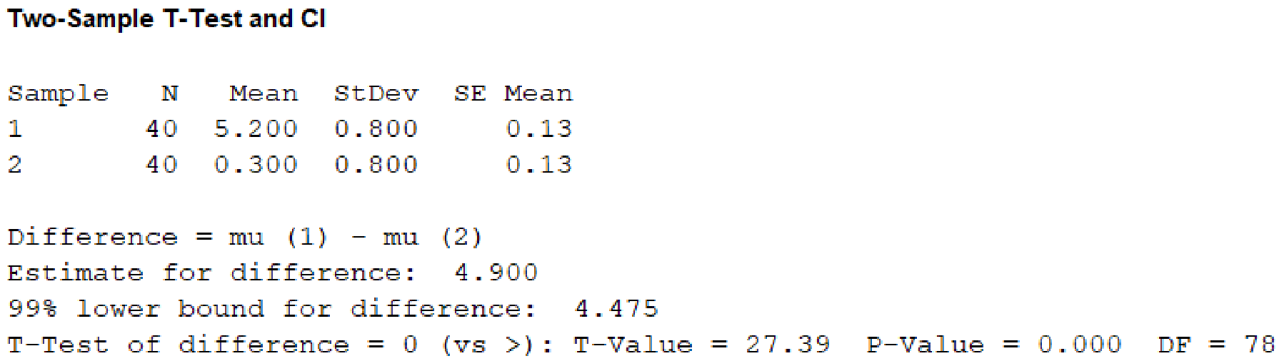
From the given MINITAB output, the value of test statistic is 27.39.
Step 8:
P-value:
From the MINITAB output, the P-value is 0.
Step 9:
Decision rule:
If the
Here, the
That is,
The decision is that the null hypothesis is rejected.
Conclusion:
Hence, there is sufficient evidence to conclude that the average number of miles per hour over the speed limit is greater for male drivers with male passengers than it is for male drivers with female passengers.
(ii)
Step 1:
In this context,
Step 2:
Null hypothesis:
Step 3:
Alternative hypothesis:
Step 4:
Significance level,
It is given that the significance level
Step 5:
Test statistic:
Step 6:
Assumptions for the two-sample t-test:
- The random samples should be collected independently.
- The sample sizes should be large. That is, each sample size must be at least 30.
Assumption in this particular problem:
- Data are collected independently.
- The sample sizes are large.
Here, both sample sizes are greater than 30.
Therefore, the assumptions are satisfied.
Step 7:
Test statistic:
Software procedure:
Step-by-step procedure to obtain the P-value and test statistic using MINITAB software:
- Choose Stat > Basic Statistics > 2 sample t.
- Choose Summarized data.
- In sample 1, enter Sample size as 40, Mean as 2.3, Standard deviation as 0.8.
- In sample 2, enter Sample size as 40, Mean as 0.6, Standard deviation as 0.8.
- Choose Options.
- In Confidence level, enter 99.
- In Alternative, select greater than.
- Click OK in all the dialogue boxes.
Output obtained using MINITAB software is given below:
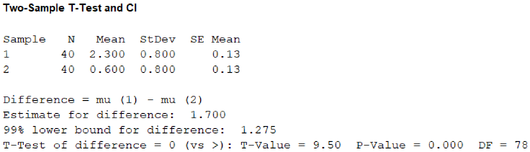
From the given MINITAB output, the value of test statistic is 9.50.
Step 8:
P-value:
From the MINITAB output, the P-value is 0.
Step 9:
Decision rule:
If the
Here, the
That is,
The decision is that the null hypothesis is rejected.
Conclusion:
Hence, there is sufficient evidence to conclude that the average number of miles per hour over the speed limit is greater for female drivers with male passengers than it is for female drivers with female passengers.
(iii)
Step 1:
In this context,
Step 2:
Null hypothesis:
Step 3:
Alternative hypothesis:
Step 4:
Significance level,
It is given that the significance level
Step 5:
Test statistic:
Step 6:
Assumptions for the two-sample t-test:
- The random samples should be collected independently.
- The sample sizes should be large. That is, each sample size must be at least 30.
Assumption in this particular problem:
- Data are collected independently.
- The sample sizes are large.
Here, both sample sizes are greater than 30.
Therefore, the assumptions are satisfied.
Step 7:
Test statistic:
Software procedure:
Step-by-step procedure to obtain the P-value and test statistic using MINITAB software:
- Choose Stat > Basic Statistics > 2 sample t.
- Choose Summarized data.
- In sample 1, enter Sample size as 40, Mean as 0.3, Standard deviation as 0.8.
- In sample 2, enter Sample size as 40, Mean as 2.3, Standard deviation as 0.8.
- Choose Options.
- In Confidence level, enter 99.
- In Alternative, select less than.
- Click OK in all the dialogue boxes.
Output obtained using the MINITAB software is given below:
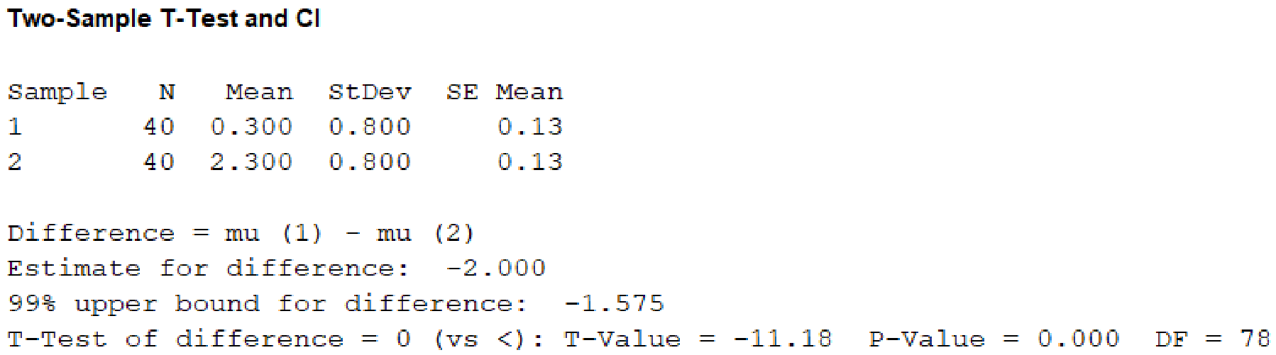
From the given MINITAB output, the value of test statistic is –11.18.
Step 8:
P-value:
From the MINITAB output, the P-value is 0.
Step 9:
Decision rule:
If the
Here, the
That is,
The decision is that the null hypothesis is rejected.
Conclusion:
Hence, there is sufficient evidence to conclude that the average number of miles per hour over the speed limit is smaller for male drivers with female passengers than it is for female drivers with male passengers.
c.
Comment on the effects of gender on teenagers driving with passengers.
c.
Explanation of Solution
Comment:
From the results, it is observed that the average speed limit for male and female drivers are greater with male passengers when compared to the female passengers. The average speed limit for male drivers are lesser with female passengers when compared to the female drivers with male passengers. The average speed limit for male drivers are greater with male passengers when compared to the female drivers with female passengers.
Want to see more full solutions like this?
Chapter 11 Solutions
Bundle: Introduction to Statistics and Data Analysis, 5th + WebAssign Printed Access Card: Peck/Olsen/Devore. 5th Edition, Single-Term


- If a uniform distribution is defined over the interval from 6 to 10, then answer the followings: What is the mean of this uniform distribution? Show that the probability of any value between 6 and 10 is equal to 1.0 Find the probability of a value more than 7. Find the probability of a value between 7 and 9. The closing price of Schnur Sporting Goods Inc. common stock is uniformly distributed between $20 and $30 per share. What is the probability that the stock price will be: More than $27? Less than or equal to $24? The April rainfall in Flagstaff, Arizona, follows a uniform distribution between 0.5 and 3.00 inches. What is the mean amount of rainfall for the month? What is the probability of less than an inch of rain for the month? What is the probability of exactly 1.00 inch of rain? What is the probability of more than 1.50 inches of rain for the month? The best way to solve this problem is begin by a step by step creating a chart. Clearly mark the range, identifying the…arrow_forwardClient 1 Weight before diet (pounds) Weight after diet (pounds) 128 120 2 131 123 3 140 141 4 178 170 5 121 118 6 136 136 7 118 121 8 136 127arrow_forwardClient 1 Weight before diet (pounds) Weight after diet (pounds) 128 120 2 131 123 3 140 141 4 178 170 5 121 118 6 136 136 7 118 121 8 136 127 a) Determine the mean change in patient weight from before to after the diet (after – before). What is the 95% confidence interval of this mean difference?arrow_forward
- In order to find probability, you can use this formula in Microsoft Excel: The best way to understand and solve these problems is by first drawing a bell curve and marking key points such as x, the mean, and the areas of interest. Once marked on the bell curve, figure out what calculations are needed to find the area of interest. =NORM.DIST(x, Mean, Standard Dev., TRUE). When the question mentions “greater than” you may have to subtract your answer from 1. When the question mentions “between (two values)”, you need to do separate calculation for both values and then subtract their results to get the answer. 1. Compute the probability of a value between 44.0 and 55.0. (The question requires finding probability value between 44 and 55. Solve it in 3 steps. In the first step, use the above formula and x = 44, calculate probability value. In the second step repeat the first step with the only difference that x=55. In the third step, subtract the answer of the first part from the…arrow_forwardIf a uniform distribution is defined over the interval from 6 to 10, then answer the followings: What is the mean of this uniform distribution? Show that the probability of any value between 6 and 10 is equal to 1.0 Find the probability of a value more than 7. Find the probability of a value between 7 and 9. The closing price of Schnur Sporting Goods Inc. common stock is uniformly distributed between $20 and $30 per share. What is the probability that the stock price will be: More than $27? Less than or equal to $24? The April rainfall in Flagstaff, Arizona, follows a uniform distribution between 0.5 and 3.00 inches. What is the mean amount of rainfall for the month? What is the probability of less than an inch of rain for the month? What is the probability of exactly 1.00 inch of rain? What is the probability of more than 1.50 inches of rain for the month? The best way to solve this problem is begin by creating a chart. Clearly mark the range, identifying the lower and upper…arrow_forwardProblem 1: The mean hourly pay of an American Airlines flight attendant is normally distributed with a mean of 40 per hour and a standard deviation of 3.00 per hour. What is the probability that the hourly pay of a randomly selected flight attendant is: Between the mean and $45 per hour? More than $45 per hour? Less than $32 per hour? Problem 2: The mean of a normal probability distribution is 400 pounds. The standard deviation is 10 pounds. What is the area between 415 pounds and the mean of 400 pounds? What is the area between the mean and 395 pounds? What is the probability of randomly selecting a value less than 395 pounds? Problem 3: In New York State, the mean salary for high school teachers in 2022 was 81,410 with a standard deviation of 9,500. Only Alaska’s mean salary was higher. Assume New York’s state salaries follow a normal distribution. What percent of New York State high school teachers earn between 70,000 and 75,000? What percent of New York State high school…arrow_forward
- Pls help asaparrow_forwardSolve the following LP problem using the Extreme Point Theorem: Subject to: Maximize Z-6+4y 2+y≤8 2x + y ≤10 2,y20 Solve it using the graphical method. Guidelines for preparation for the teacher's questions: Understand the basics of Linear Programming (LP) 1. Know how to formulate an LP model. 2. Be able to identify decision variables, objective functions, and constraints. Be comfortable with graphical solutions 3. Know how to plot feasible regions and find extreme points. 4. Understand how constraints affect the solution space. Understand the Extreme Point Theorem 5. Know why solutions always occur at extreme points. 6. Be able to explain how optimization changes with different constraints. Think about real-world implications 7. Consider how removing or modifying constraints affects the solution. 8. Be prepared to explain why LP problems are used in business, economics, and operations research.arrow_forwardged the variance for group 1) Different groups of male stalk-eyed flies were raised on different diets: a high nutrient corn diet vs. a low nutrient cotton wool diet. Investigators wanted to see if diet quality influenced eye-stalk length. They obtained the following data: d Diet Sample Mean Eye-stalk Length Variance in Eye-stalk d size, n (mm) Length (mm²) Corn (group 1) 21 2.05 0.0558 Cotton (group 2) 24 1.54 0.0812 =205-1.54-05T a) Construct a 95% confidence interval for the difference in mean eye-stalk length between the two diets (e.g., use group 1 - group 2).arrow_forward
- An article in Business Week discussed the large spread between the federal funds rate and the average credit card rate. The table below is a frequency distribution of the credit card rate charged by the top 100 issuers. Credit Card Rates Credit Card Rate Frequency 18% -23% 19 17% -17.9% 16 16% -16.9% 31 15% -15.9% 26 14% -14.9% Copy Data 8 Step 1 of 2: Calculate the average credit card rate charged by the top 100 issuers based on the frequency distribution. Round your answer to two decimal places.arrow_forwardPlease could you check my answersarrow_forwardLet Y₁, Y2,, Yy be random variables from an Exponential distribution with unknown mean 0. Let Ô be the maximum likelihood estimates for 0. The probability density function of y; is given by P(Yi; 0) = 0, yi≥ 0. The maximum likelihood estimate is given as follows: Select one: = n Σ19 1 Σ19 n-1 Σ19: n² Σ1arrow_forward
 Glencoe Algebra 1, Student Edition, 9780079039897...AlgebraISBN:9780079039897Author:CarterPublisher:McGraw Hill
 Big Ideas Math A Bridge To Success Algebra 1: Stu...AlgebraISBN:9781680331141Author:HOUGHTON MIFFLIN HARCOURTPublisher:Houghton Mifflin Harcourt
 College Algebra (MindTap Course List)AlgebraISBN:9781305652231Author:R. David Gustafson, Jeff HughesPublisher:Cengage Learning
 Holt Mcdougal Larson Pre-algebra: Student Edition...AlgebraISBN:9780547587776Author:HOLT MCDOUGALPublisher:HOLT MCDOUGAL