
Videos
a.
Check whether there is evidence that there is a difference in the
a.
Answer to Problem 48DE
The conclusion is that there is no evidence of a difference in the mean salary of teams in the American League versus teams in the National League.
Explanation of Solution
In this context, let
The hypotheses are given below:
Null hypothesis:
Alternative hypothesis:
Significance level,
It is given that the significance level,
Degrees of freedom:
The degrees of freedom is as follows:
Step-by-step procedure to obtain the critical values using MINITAB software:
- Choose Graph > Probability Distribution Plot choose View Probability > OK.
- From Distribution, choose ‘t’ distribution.
- In Degrees of freedom, enter 28.
- Click the Shaded Area tab.
- Choose Probability and Both Tails for the region of the curve to shade.
- Enter the Probability as 0.05.
- Click OK.
Output obtained using MINITAB software is given below:
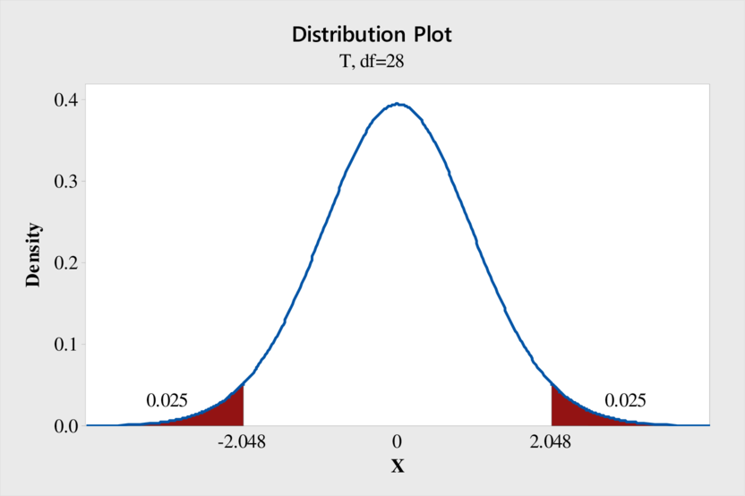
From the MINITAB output, the critical values are
The decision rule is as follows:
If
If
If
Test statistic:
Step-by-step procedure to obtain the P-value and test statistic using MINITAB software:
- Choose Stat > Basic Statistics > 2 sample t.
- Choose Each sample in its own column.
- In Sample 1, enter the column of American.
- In Sample 2, enter the column of National.
- Choose Assume equal variance.
- Choose Options.
- In Confidence level, enter 95.
- In Alternative, select not equal.
- Click OK in all the dialogue boxes.
Output obtained using MINITAB software is given below:
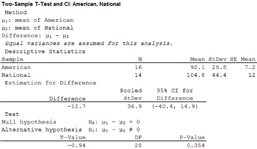
From the given MINITAB output, the value of the test statistic is –0.94.
Decision:
The value of test statistic lies between the critical values.
From the decision rule, fail to reject the null hypothesis.
Therefore, there is no evidence of a difference in the mean salary of teams in the American League versus teams in the National League.
b.
Check whether there is evidence that there is a difference in the mean home attendance of team in the American League versus teams in the National League.
b.
Answer to Problem 48DE
The conclusion is that there is no evidence of a difference in the mean home attendance of teams in the American League versus teams in the National League.
Explanation of Solution
In this context, let
The hypotheses are given below:
Null hypothesis:
Alternative hypothesis:
Significance level,
It is given that the significance level,
From the MINITAB output in Part (a), the critical values are
Test statistic:
Step-by-step procedure to obtain the P-value and test statistic using MINITAB software:
- Choose Stat > Basic Statistics > 2 sample t.
- Choose Each sample in its own column.
- In Sample 1, enter the column of American.
- In Sample 2, enter the column of National.
- Choose Assume equal variance.
- Choose Options.
- In Confidence level, enter 95.
- In Alternative, select not equal.
- Click OK in all the dialogue boxes.
Output obtained using MINITAB software is given below:
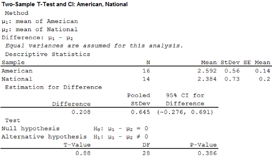
From the given MINITAB output, the value of the test statistic is 0.88.
Decision:
The value of test statistic lies between the critical values.
From the decision rule, fail to reject the null hypothesis.
Therefore, there is no evidence of a difference in the mean home attendance of teams in the American League versus teams in the National League.
c.
Check whether there is evidence of a difference in the mean number of wins for teams in the American League versus teams in the National League.
c.
Answer to Problem 48DE
The conclusion is that there is no evidence of difference in the mean number of wins for teams in the American League versus teams in the National League.
Explanation of Solution
In this context, let
The hypotheses are given below:
Null hypothesis:
Alternative hypothesis:
Significance level,
It is given that the significance level,
Degrees of freedom:
The degrees of freedom is as follows:
Step-by-step procedure to obtain the critical values using MINITAB software:
- Choose Graph > Probability Distribution Plot choose View Probability > OK.
- From Distribution, choose ‘t’ distribution.
- In Degrees of freedom, enter 18.
- Click the Shaded Area tab.
- Choose Probability and Both Tails for the region of the curve to shade.
- Enter the Probability as 0.05.
- Click OK.
Output obtained using MINITAB software is given below:
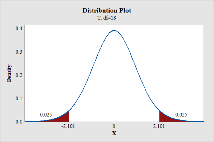
From the MINITAB output, the critical values are
The decision rule is as follows:
If
If
If
Test statistic:
Step-by-step procedure to obtain the P-value and test statistic using MINITAB software:
- Choose Stat > Basic Statistics > 2 sample t.
- Choose Each sample in its own column.
- In Sample 1, enter the column of American.
- In Sample 2, enter the column of National.
- Choose Assume equal variance.
- Choose Options.
- In Confidence level, enter 95.
- In Alternative, select not equal.
- Click OK in all the dialogue boxes.
Output obtained using MINITAB software is given below:
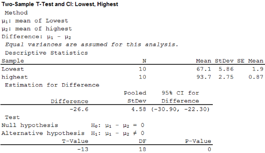
From the given MINITAB output, the value of the test statistic is –13.
Decision:
The value of test statistic does not lie between the critical values.
That is,
From the decision rule, reject the null hypothesis.
Therefore, there is evidence of a difference in the mean number of wins for teams in the American League versus teams in the National League.
Want to see more full solutions like this?
Chapter 11 Solutions
Loose Leaf for Statistical Techniques in Business and Economics (Mcgraw-hill/Irwin Series in Operations and Decision Sciences)


- For a binary asymmetric channel with Py|X(0|1) = 0.1 and Py|X(1|0) = 0.2; PX(0) = 0.4 isthe probability of a bit of “0” being transmitted. X is the transmitted digit, and Y is the received digit.a. Find the values of Py(0) and Py(1).b. What is the probability that only 0s will be received for a sequence of 10 digits transmitted?c. What is the probability that 8 1s and 2 0s will be received for the same sequence of 10 digits?d. What is the probability that at least 5 0s will be received for the same sequence of 10 digits?arrow_forwardV2 360 Step down + I₁ = I2 10KVA 120V 10KVA 1₂ = 360-120 or 2nd Ratio's V₂ m 120 Ratio= 360 √2 H I2 I, + I2 120arrow_forwardQ2. [20 points] An amplitude X of a Gaussian signal x(t) has a mean value of 2 and an RMS value of √(10), i.e. square root of 10. Determine the PDF of x(t).arrow_forward
- In a network with 12 links, one of the links has failed. The failed link is randomlylocated. An electrical engineer tests the links one by one until the failed link is found.a. What is the probability that the engineer will find the failed link in the first test?b. What is the probability that the engineer will find the failed link in five tests?Note: You should assume that for Part b, the five tests are done consecutively.arrow_forwardProblem 3. Pricing a multi-stock option the Margrabe formula The purpose of this problem is to price a swap option in a 2-stock model, similarly as what we did in the example in the lectures. We consider a two-dimensional Brownian motion given by W₁ = (W(¹), W(2)) on a probability space (Q, F,P). Two stock prices are modeled by the following equations: dX = dY₁ = X₁ (rdt+ rdt+0₁dW!) (²)), Y₁ (rdt+dW+0zdW!"), with Xo xo and Yo =yo. This corresponds to the multi-stock model studied in class, but with notation (X+, Y₁) instead of (S(1), S(2)). Given the model above, the measure P is already the risk-neutral measure (Both stocks have rate of return r). We write σ = 0₁+0%. We consider a swap option, which gives you the right, at time T, to exchange one share of X for one share of Y. That is, the option has payoff F=(Yr-XT). (a) We first assume that r = 0 (for questions (a)-(f)). Write an explicit expression for the process Xt. Reminder before proceeding to question (b): Girsanov's theorem…arrow_forwardProblem 1. Multi-stock model We consider a 2-stock model similar to the one studied in class. Namely, we consider = S(1) S(2) = S(¹) exp (σ1B(1) + (M1 - 0/1 ) S(²) exp (02B(2) + (H₂- M2 where (B(¹) ) +20 and (B(2) ) +≥o are two Brownian motions, with t≥0 Cov (B(¹), B(2)) = p min{t, s}. " The purpose of this problem is to prove that there indeed exists a 2-dimensional Brownian motion (W+)+20 (W(1), W(2))+20 such that = S(1) S(2) = = S(¹) exp (011W(¹) + (μ₁ - 01/1) t) 롱) S(²) exp (021W (1) + 022W(2) + (112 - 03/01/12) t). where σ11, 21, 22 are constants to be determined (as functions of σ1, σ2, p). Hint: The constants will follow the formulas developed in the lectures. (a) To show existence of (Ŵ+), first write the expression for both W. (¹) and W (2) functions of (B(1), B(²)). as (b) Using the formulas obtained in (a), show that the process (WA) is actually a 2- dimensional standard Brownian motion (i.e. show that each component is normal, with mean 0, variance t, and that their…arrow_forward
- The scores of 8 students on the midterm exam and final exam were as follows. Student Midterm Final Anderson 98 89 Bailey 88 74 Cruz 87 97 DeSana 85 79 Erickson 85 94 Francis 83 71 Gray 74 98 Harris 70 91 Find the value of the (Spearman's) rank correlation coefficient test statistic that would be used to test the claim of no correlation between midterm score and final exam score. Round your answer to 3 places after the decimal point, if necessary. Test statistic: rs =arrow_forwardBusiness discussarrow_forwardBusiness discussarrow_forward
 Glencoe Algebra 1, Student Edition, 9780079039897...AlgebraISBN:9780079039897Author:CarterPublisher:McGraw Hill
 Big Ideas Math A Bridge To Success Algebra 1: Stu...AlgebraISBN:9781680331141Author:HOUGHTON MIFFLIN HARCOURTPublisher:Houghton Mifflin Harcourt
 Holt Mcdougal Larson Pre-algebra: Student Edition...AlgebraISBN:9780547587776Author:HOLT MCDOUGALPublisher:HOLT MCDOUGAL